Journal of Fluid Flow, Heat and Mass Transfer (JFFHMT)
ISSN: 2368-6111

Volume 12 - Year 2025 - Pages 404-416
DOI: 10.11159/jffhmt.2025.040
Stagnation-Point Flow of Williamson Fluid: A Study on Dual Solutions and Stability Analysis
Dibjyoti Mondal1, Abhijit Das1
1 Department of Mathematics, National Institute of Technology Tiruchirappalli,
Tiruchirappalli, Tamil Nadu-620015, India
dibjyoti002121@gmail.com
Abstract - Since non-Newtonian fluids are often encountered in engineering devices, the nonlinear boundary layer equations governing the flow and heat transfer properties of a non-Newtonian Williamson fluid over a stretching (c>0) or shrinking (c<0) sheet near the stagnation point are analyzed using two closely interrelated approaches. First, employing the shooting argument, it is proved that a unique solution exists when c∈ (-1,∞) and second, using the BVP4C solver in MATLAB, two different solution branches are reported on the interval [cT,-1], where cT is the bifurcation point. The cT values become more negative with increasing values of the Williamson parameter λ, marking the broadening of the solution range. Furthermore, the first solution branch continues for large positive values of c, whereas the second branch seems to cease at F''(0)=0 as c→-1. The smallest eigenvalue computed using temporal stability analysis of these solutions is found to be positive for the first branch, indicating that this branch is physically stable. These findings are relevant to various industrial processes involving non-Newtonian fluids, such as polymer processing and coating applications. Finally, an asymptotic expression is derived to provide insights into the behavior of large c.
Keywords: Williamson fluid, Existence-Uniqueness, Dual solutions, Stability analysis, Asymptotic analysis.
© Copyright 2025 Authors - This is an Open Access article published under the Creative Commons Attribution License terms Creative Commons Attribution License terms. Unrestricted use, distribution, and reproduction in any medium are permitted, provided the original work is properly cited.
Date Received: 2025-05-26
Date Revised: 2025-09-23
Date Accepted: 2025-10-09
Date Published: 2025-12-01
1. Introduction
It is common knowledge that many industrial (such as paints and coatings) and physiological (such as blood and plasma) fluids exhibit complex flow behavior that the classical Newtonian fluid model cannot adequately describe. To gain a better understanding of such fluids, numerous models (non-Newtonian) have been suggested over the years to take into account the unique characteristics of these fluids, including their viscoelastic properties, shear-thinning or shear-thickening behavior, and time-dependent responses [1, 2]. The nonlinear relationships between the stress tensor and the deformation rate tensor for non-Newtonian fluids give rise to complex equations. Undoubtedly, it is challenging to prove the existence and uniqueness/non-uniqueness of a solution to these equations and obtain their numerical solution.
This paper focuses on the robust model put forward by Williamson to describe pseudoplastic fluids [3]. A large number of published works, for example, the study of the flow of a thin layer of pseudoplastic fluid over an inclined solid surface [4], the peristaltic flow of chyme in the small intestine [5], blood flows through a tapered artery with stenosis [6], and some boundary layer flows of Williamson fluid [7], to mention a few, demonstrate the adequacy of Williamson's model in describing many frequently observed industrial and physiological fluids like polymer solutions, paints, blood, and plasma. Further, one can go through the investigations [8, 9] for Williamson fluid flows in various geometries (especially stagnation point flow and stretching/shrinking surface) under diverse physical conditions. Due to its immense engineering and industrial applications, the stagnation-point flow of a viscous or non-Newtonian fluid has been the subject of several investigations [10, 11]. Another significant aspect of boundary layer flow involves the stretching or shrinking phenomena [12].
A review of the literature suggests that the flow generated by a shrinking sheet has recently captured the interest of researchers due to its intriguing physical characteristics and growing practical implementations. Wang [11] introduced the concept of flow resulting from a shrinking sheet and showed that the solution is not unique to a particular domain. Subsequently, several research papers [13-15] have been published addressing the shrinking sheet problem. The works mentioned above were devoted to finding multiple solutions and their stability analysis. Analyzing multiple solutions and stability is crucial in engineering analysis as it enables the determination of the physical relevance of a steady-state solution. In the context of stability analysis, Merkin [16] first found that in time-dependent problems of steady-state flows, only the stable upper branch solution is physically possible, as it has the smallest positive eigenvalue. In contrast, the unstable lower branch solution is not physically relevant. Recent studies in references [17, 18] have discussed the stability of multiple solutions associated with stretching or shrinking surfaces.
In the last few decades,
numerous investigations have demonstrated the mathematical proof of the
existence and uniqueness of solutions in boundary layer fluid flow problems.
Miklavčič and Wang [19] established the existence and uniqueness of the
similarity solution for the equation describing the flow caused by a shrinking
sheet with suction. Gorder et al. [20] examined the results concerning the
existence and uniqueness of solutions over the interval ![]() for the stagnation-point flow of a hydromagnetic
fluid over a stretching or shrinking sheet. Pallet et al. [10] proved the
existence and uniqueness of a solution for oblique stagnation point flow by
using the topological shooting argument.However, to the best of
the authors' knowledge, only a limited number of articles are devoted to
answering the question of the existence of a unique solution, see [21, 22, 23]
and the references therein for a detailed understanding of the methodology
used.
for the stagnation-point flow of a hydromagnetic
fluid over a stretching or shrinking sheet. Pallet et al. [10] proved the
existence and uniqueness of a solution for oblique stagnation point flow by
using the topological shooting argument.However, to the best of
the authors' knowledge, only a limited number of articles are devoted to
answering the question of the existence of a unique solution, see [21, 22, 23]
and the references therein for a detailed understanding of the methodology
used.
Motivated by the investigations mentioned above and recognizing the widespread applications of problems involving stretching/shrinking sheets and non-Newtonian fluids in engineering and industries, we consider the stagnation point flow of the Williamson fluid model over a stretching/shrinking surface here. Primarily, the following research questions are addressed
·
How
can the existence and uniqueness of solutions for the stretching/shrinking
parameter ![]() be
mathematically established?
be
mathematically established?
·
What
is the critical point ![]() and
how does the nature of the solution change when
and
how does the nature of the solution change when ![]()
·
What
are the characteristics of dual solutions in the shrinking parameter range ![]() ?
?
· How can a linear stability analysis be conducted to identify stable solutions?
·
What
are the effects of the non-Newtonian parameter ![]() and shrinking parameter
and shrinking parameter ![]() (specifically
(specifically ![]() )
on the velocity and temperature profiles in the dual solution?
)
on the velocity and temperature profiles in the dual solution?
·
How
do the expressions for shear stresses and the Nusselt number behave for large ![]() ?
?
2. Flow Analysis
The continuity and momentum equations for an incompressible Williamson fluid are expressed as follows [7]

The energy equation is
![]()
Here, ![]() represents the velocity vector,
represents the velocity vector, ![]() denotes the
temperature,
denotes the
temperature, ![]() stands for
density,
stands for
density, ![]() denotes the
body force,
denotes the
body force, ![]() signifies the material time derivative,
signifies the material time derivative, ![]() represents
pressure,
represents
pressure, ![]() indicates the specific heat,
indicates the specific heat, ![]() represent the
thermal conductivity and
represent the
thermal conductivity and ![]() be the
identity matrix.
be the
identity matrix. ![]() be anisotropic
viscous stress tensor defined as [7]
be anisotropic
viscous stress tensor defined as [7]
![]()
Here ![]() and
and ![]() be zero and infinity shear rate viscosity, respectively,
be zero and infinity shear rate viscosity, respectively,
![]() be the first Rivlin-Erickson tensor,
be the first Rivlin-Erickson tensor, ![]() be the time
constant and
be the time
constant and ![]() is defined as
is defined as

As in [7], we
investigate the circumstance where ![]() and
and ![]() . Under this variation, (4) transforms into
. Under this variation, (4) transforms into
![]()
Consider a steady,
two-dimensional, incompressible flow of a Williamson fluid over a horizontal
linearly stretching/shrinking sheet with no body force. The sheet, which
coincides with the plane ![]() , is assumed to be impermeable, so there is
no normal velocity across its surface. The flow is restricted to the area where
, is assumed to be impermeable, so there is
no normal velocity across its surface. The flow is restricted to the area where
![]() . The sheet's velocity is represented by
. The sheet's velocity is represented by ![]() , where
, where ![]() (where
(where ![]() ) characterizes the free stream velocity. Here,
the constant
) characterizes the free stream velocity. Here,
the constant ![]() represents stretching and
represents stretching and ![]() represents shrinking. Let (
represents shrinking. Let (![]() ) be the velocity component in
) be the velocity component in ![]() direction and
direction and ![]() be the
temperature. Following [7], the boundary layer equations are expressed as
be the
temperature. Following [7], the boundary layer equations are expressed as
![]()
and
![]()
Relevant boundary conditions for the stagnation point flow of Williamson fluid over a stretching/shrinking sheet [7] are
![]()
where ![]() and
and ![]() are the surface and ambient temperature,
respectively. Using the Bernoulli equation and neglecting the hydrostatic term,
are the surface and ambient temperature,
respectively. Using the Bernoulli equation and neglecting the hydrostatic term,
![]() , gives
, gives ![]() .
.
Following the similarity transformations ![]() [7], where
[7], where ![]() ,
,
the equations (7)-(8) become
![]()
where ![]() be the non-Newtonian Williamson parameter and
be the non-Newtonian Williamson parameter and ![]() is the Prandtl number. Also, the boundary
conditions (9)-(10) become
is the Prandtl number. Also, the boundary
conditions (9)-(10) become
![]()
![]() (13)
(13)
where ![]() represents
the stretching
represents
the stretching ![]() or
shrinking
or
shrinking ![]() parameter.
Wall suction and injection effects are neglected in this study (
parameter.
Wall suction and injection effects are neglected in this study (![]() ).
).
The coefficient
of skin friction ![]() and the Nusselt number
and the Nusselt number ![]() , which are two crucial physical parameters, are
outlined below
, which are two crucial physical parameters, are
outlined below
![]()
Here, ![]() represents the skin friction or shear stress
along the stretching/shrinking surface, and
represents the skin friction or shear stress
along the stretching/shrinking surface, and ![]() denotes the heat flux originating from the
stretching/shrinking surface. These quantities are specified as follows
denotes the heat flux originating from the
stretching/shrinking surface. These quantities are specified as follows
![]()
![]()
After using the similarity transformation, equation (14) becomes
![]()
![]() (15)
(15)
where ![]() is the Reynolds number.
is the Reynolds number.
3. Existence and
uniqueness results for ![]()
3.1 Existence for ![]()
The existence of a
solution for the boundary value problem in equations (11)-(13) is analyzed
using the topological shooting
method. This method entails the investigation of a corresponding group of
initial value problems (IVP), denoted as the ODE (11) and (13) (except the
condition at ![]() ), in conjunction with an additional initial
condition specified as
), in conjunction with an additional initial
condition specified as ![]() , where
, where ![]() can take any
arbitrary values. Then, the solution of the IVP depends on both
can take any
arbitrary values. Then, the solution of the IVP depends on both ![]() and
and ![]() and is denoted
as
and is denoted
as ![]() . Although each
. Although each ![]() yields a
solution for the IVP, not all these solutions will satisfy the boundary
conditions (13). Therefore, it is necessary to determine a suitable value for
yields a
solution for the IVP, not all these solutions will satisfy the boundary
conditions (13). Therefore, it is necessary to determine a suitable value for ![]() that satisfies
the condition at
that satisfies
the condition at ![]() . To prove the existence of a solution, the range
. To prove the existence of a solution, the range ![]() is divided into two parts:
is divided into two parts: ![]() and
and ![]() . For
. For ![]() , the identity function
, the identity function ![]() is a solution of (11). In this case
is a solution of (11). In this case ![]() for all
for all ![]() , therefore, we
did not consider the case
, therefore, we
did not consider the case ![]() in our proof.
in our proof.
3.1.1
Existence Proof for ![]()
Let us assume
two sets ![]() and
and ![]() are subsets of
are subsets of ![]() , defined by
, defined by
![]()
![]() (16)
(16)
Lemma 1. ![]() and
and
![]() are
open sets with no elements in common.
are
open sets with no elements in common.
Proof: Clearly ![]() and
and ![]() have no element in common. Let
have no element in common. Let ![]() then
then ![]() such that
such that ![]() and
and ![]() for
for ![]()
![]() . Since
. Since ![]() , therefore, using the property of continuous
functions
, therefore, using the property of continuous
functions ![]() a neighborhood
of
a neighborhood
of ![]() such that for all points in the neighborhood,
such that for all points in the neighborhood, ![]() have the same sign as
have the same sign as ![]() . Thus
. Thus ![]() has a root with
has a root with ![]() . This shows that
. This shows that ![]() is an open set. Similarly, one can prove that
is an open set. Similarly, one can prove that ![]() is open as well.
is open as well.
Lemma 2. ![]() is
non-void.
is
non-void.
Proof: We claim that when ![]() is very small,
it is in
is very small,
it is in ![]() . Let
. Let ![]() , then
, then ![]() for all
for all ![]() . Thus, in a
small enough vicinity around
. Thus, in a
small enough vicinity around ![]() , it holds that
, it holds that ![]() and
and ![]() . Then, through the continuous solutions of the
IVP, along with its initial conditions, there is a positive number
. Then, through the continuous solutions of the
IVP, along with its initial conditions, there is a positive number ![]() for which
for which ![]() and
and ![]() hold for all values of
hold for all values of ![]() in the
vicinity of
in the
vicinity of ![]() . But
. But ![]() , implies
, implies ![]() a
a ![]() such that
such that ![]() and
and ![]() for
for ![]() . Hence for small
. Hence for small ![]() , it is in
, it is in ![]() .
.
Lemma 3. ![]() is
non-void.
is
non-void.
Proof: We claim that when ![]() is very large,
it is in
is very large,
it is in ![]() , that is
, that is ![]() in
in ![]() strictly before
strictly before ![]() . If this is not the case, then the following
possibilities must occur : (i)
. If this is not the case, then the following
possibilities must occur : (i) ![]() for some point in
for some point in ![]() for which
for which ![]() , (ii)
, (ii) ![]() and
and ![]() in
in ![]() , and (iii)
, and (iii) ![]() and
and ![]() occur concurrently. If possible, let
occur concurrently. If possible, let ![]() such that
such that ![]() with
with ![]() for
for ![]() . By integrating, we get
. By integrating, we get ![]() . Now let
. Now let ![]() and integrating (11) from 0 to
and integrating (11) from 0 to ![]() , we get
, we get
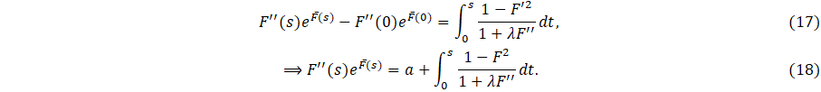
Let ![]() , then form (18) we have
, then form (18) we have
![]()
Then
for ![]()
![]()
Thus, for large ![]() for all
for all ![]() , leading to a
contradiction. Similarly, it can be shown that the second statement cannot
occur for sufficiently large values of
, leading to a
contradiction. Similarly, it can be shown that the second statement cannot
occur for sufficiently large values of ![]() . If the third
case occurs, then from (11), we get
. If the third
case occurs, then from (11), we get ![]() . That implies that
. That implies that ![]() , which contradicts the fact that
, which contradicts the fact that ![]() . Therefore, sufficiently large
. Therefore, sufficiently large ![]() belongs to
belongs to ![]() .
.
Theorem 1. For any ![]() ,
equations (11) and (13) have a solution. Also, the solution is monotone in nature.
,
equations (11) and (13) have a solution. Also, the solution is monotone in nature.
Proof: As ![]() is a connected set, and both
is a connected set, and both ![]() and
and ![]() are non-empty, open, and disjoint from each
other, it follows from the definition of a connected set that the union of
are non-empty, open, and disjoint from each
other, it follows from the definition of a connected set that the union of ![]() and
and ![]() cannot be equal to
cannot be equal to ![]() . Therefore
. Therefore ![]() such that
such that ![]() and
and ![]() . Also, Lemma 3 implies that
. Also, Lemma 3 implies that ![]() and
and ![]() do not occur simultaneously. Consequently, there
is only one possibility that
do not occur simultaneously. Consequently, there
is only one possibility that ![]() and
and ![]() . Now, from equation (11), it is observed that as
. Now, from equation (11), it is observed that as ![]() approaches 1, implies the existence of a
monotonically increasing solution to the boundary value problem (11), (13).
approaches 1, implies the existence of a
monotonically increasing solution to the boundary value problem (11), (13).
3.1.2 Existence
Proof for ![]()
Let us assume two sets ![]() and
and ![]() are subsets of
are subsets of ![]() , defined by
, defined by
![]() ,
,
![]() .
.
As mentioned in the
previous subsection, we will show the same properties (Lemma 1-3) of the sets ![]() and
and ![]() . To show
. To show ![]() and
and ![]() are open is the same as the previous proof, so we
skip this. To prove
are open is the same as the previous proof, so we
skip this. To prove ![]() is non-void, we will show that if
is non-void, we will show that if ![]() and
and ![]() is very small, it belongs to
is very small, it belongs to ![]() . Now, from (13), first we take
. Now, from (13), first we take ![]() and subsequently, at
and subsequently, at ![]() ,
,
![]()
So we can say that if ![]() is close to 0
then
is close to 0
then ![]() 0 and
0 and ![]() . By continuous solution of the IVP, for
. By continuous solution of the IVP, for ![]() with sufficiently small magnitude, it is evident
that
with sufficiently small magnitude, it is evident
that ![]() will be close to
will be close to ![]() . Specifically,
. Specifically, ![]() with
with ![]() , but
, but ![]() based on equation (13). This implies that there exists
based on equation (13). This implies that there exists
![]() where
where ![]() , and
, and ![]() whenever
whenever ![]() , showing that the set
, showing that the set ![]() is non-empty.
is non-empty.
Next, we will prove that ![]() is non-empty. For that, first, we integrate
equation (11) from 0 to
is non-empty. For that, first, we integrate
equation (11) from 0 to ![]() which gives
which gives

We claim that for large ![]() , it is in
, it is in ![]() . If possible, let the statement mentioned above
be false, then at least one among the following options is necessary: (i)
. If possible, let the statement mentioned above
be false, then at least one among the following options is necessary: (i) ![]() at some point in
at some point in ![]() with
with ![]() . (ii)
. (ii) ![]() and
and ![]() for all
for all ![]() in
in ![]() . (iii)
. (iii) ![]() and
and ![]() occurs at the same time. Now, we need to refute
each of these statements. Starting with (i), let's assume that
occurs at the same time. Now, we need to refute
each of these statements. Starting with (i), let's assume that ![]() such that
such that ![]() with
with ![]() for
for ![]() . After integrating, we have
. After integrating, we have ![]() . From (23), we can write
. From (23), we can write

We are establishing some
inequalities to find the bounds of ![]() : (a) since
: (a) since ![]() , implies that
, implies that ![]() , (b) For
, (b) For ![]() implies that
implies that ![]() , also
, also ![]() implies that
implies that ![]() . After applying the inequalities (a)-(b) in (24),
we have
. After applying the inequalities (a)-(b) in (24),
we have
![]()
Now, if we assume that ![]() , then (25) gives
, then (25) gives ![]() , which is a contradiction. So (i) can not happen.
Similarly, if we take
, which is a contradiction. So (i) can not happen.
Similarly, if we take ![]() , then (ii) can not happen. If (iii) occurs, then
from (13) we have
, then (ii) can not happen. If (iii) occurs, then
from (13) we have ![]() implying that
implying that ![]() which contradicts the existence theorem of IVP as
which contradicts the existence theorem of IVP as
![]() . Hence, if
. Hence, if ![]() , then
, then ![]() before
before ![]() , implies
, implies ![]() and
and ![]() is non-empty.
is non-empty.
The sets U and V open, and mutually exclusive. Since ![]() is a connected set, therefore
is a connected set, therefore ![]() . Hence, there exists
. Hence, there exists ![]() that is not in
that is not in ![]() or
or ![]() . For that particular value of
. For that particular value of ![]() , the only option is
, the only option is ![]() and
and ![]()
![]() for
for ![]() . Therefore
. Therefore ![]()
![]() (finite). Now, from (11), we get
(finite). Now, from (11), we get ![]() which completes the proof.
which completes the proof.
3.1.3
Uniqueness Proof for ![]()
Theorem 2. For any ![]() ,
the solution is unique.
,
the solution is unique.
Proof: We will prove this theorem by using the method of
contradiction. Let us assume that ![]() ,
, ![]() (values of
(values of ![]() such that
such that ![]() and
and ![]() are the corresponding solutions. Apply MVT on the
function
are the corresponding solutions. Apply MVT on the
function ![]() in the interval
in the interval ![]() and as
and as![]() then
then ![]() such that
such that ![]() . Next, let
. Next, let ![]() and differentiating (11) and using the boundary
conditions (13), we have
and differentiating (11) and using the boundary
conditions (13), we have
![]() ,
(26)
,
(26)
with
![]()
![]() .
.
(27)
Further differentiating (26), we have
![]() .
(28)
.
(28)
Now, from (27), we can say
that ![]() such that
such that ![]() for
for ![]() . Specifically, the function
. Specifically, the function ![]() is convex downwards, initially increasing, and it
has a maximum value to reach zero. Let the maximum value occur at
is convex downwards, initially increasing, and it
has a maximum value to reach zero. Let the maximum value occur at ![]() . Consequently,
. Consequently, ![]() and
and ![]() for
for ![]() . Also,
. Also, ![]() . But equation (28) implies
. But equation (28) implies
![]() (29)
(29)
a
contradiction. However, up until the point ![]() and all its derivatives up to
and all its derivatives up to ![]() are growing positively. Hence,
are growing positively. Hence, ![]() and all its derivatives up to
and all its derivatives up to ![]() are increasing functions. Therefore, for any
are increasing functions. Therefore, for any ![]() in the
interval
in the
interval ![]() ,
, ![]() which contradicts the MVT of
which contradicts the MVT of ![]() . Hence, the proof is complete.
. Hence, the proof is complete.
3.1.4
Uniqueness Proof for ![]()
The proof part is similar
to Theorem 2. As in Theorem 2, we define ![]() , which satisfies the equation (30) and the
boundary conditions
, which satisfies the equation (30) and the
boundary conditions ![]()
![]() . Here, we observe that
. Here, we observe that ![]() and
and ![]() are first positive and increasing. Suppose there
exist two solutions corresponding to
are first positive and increasing. Suppose there
exist two solutions corresponding to ![]() (values of
(values of ![]() . We first prove that
. We first prove that ![]() cannot have a maximum value. If possible, suppose
that
cannot have a maximum value. If possible, suppose
that ![]() has a maximum at
has a maximum at ![]() and at this point, we get
and at this point, we get ![]() and
and ![]() . Moreover, for
. Moreover, for ![]() , we have
, we have
![]()
Now from (30), we get
![]()
![]() (32)
(32)
which
contradicts that ![]() . Therefore,
. Therefore, ![]() cannot have a maximum, and a positive
cannot have a maximum, and a positive ![]() and
and ![]() exists for which
exists for which ![]() is greater than
is greater than ![]() for all
for all ![]() beyond
beyond ![]() . Applying MVT, we can write for
. Applying MVT, we can write for ![]()
![]()
As ![]() in (33) gives a contradiction (left-hand side is
0 and right-hand side is always positive), demonstrating that for
in (33) gives a contradiction (left-hand side is
0 and right-hand side is always positive), demonstrating that for ![]() , there cannot be two solutions.
, there cannot be two solutions.
3.2
Existence for ![]() :
:
Theorem 3. If ![]() is a twice differentiable function satisfying (12)
with boundary condition (13), then
is a twice differentiable function satisfying (12)
with boundary condition (13), then ![]() is of the form
is of the form

4 Numerical Solution
In this section, we are
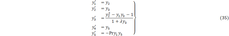
solving (11)-(13) numerically by the BVP4C solver in MATLAB. Now, equations (11)-(13)
can be written as a system of first-order initial value problems. For that let ![]() then from (11)-(13), we can obtain
then from (11)-(13), we can obtain
with
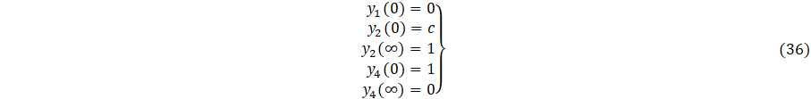
Now, we can solve equation
(35) along with the boundary conditions (36). To obtain the value of ![]() we need to choose initial values and use them to
solve for
we need to choose initial values and use them to
solve for ![]() and
and ![]() . The MATLAB solver
BVP4C was employed with a mesh of 400 points, a relative tolerance of
. The MATLAB solver
BVP4C was employed with a mesh of 400 points, a relative tolerance of ![]() , and an absolute tolerance of
, and an absolute tolerance of ![]() . The far-field boundary was truncated at
. The far-field boundary was truncated at ![]() , ensuring that velocity and temperature gradients
approached zero. Numerically, it is seen that within a specific range of
, ensuring that velocity and temperature gradients
approached zero. Numerically, it is seen that within a specific range of ![]() , there are two
sets of solutions for different values of
, there are two
sets of solutions for different values of ![]() . Determining
an initial estimate for the first solution is relatively straightforward since
the BVP4C method converges to the first solution even
with sub-optimal guesses. However, generating a suitablyaccurate
estimate for the solution becomes challenging in the case of opposing flow. To
address this challenge, we initiate the process with a group of parameter values
that make the problem easily solvable. Subsequently, we employ the acquired
outcome as the initial estimate for solving the problem with slight parameter
variations. This process is reiterated until the accurate parameter values are
attained.
. Determining
an initial estimate for the first solution is relatively straightforward since
the BVP4C method converges to the first solution even
with sub-optimal guesses. However, generating a suitablyaccurate
estimate for the solution becomes challenging in the case of opposing flow. To
address this challenge, we initiate the process with a group of parameter values
that make the problem easily solvable. Subsequently, we employ the acquired
outcome as the initial estimate for solving the problem with slight parameter
variations. This process is reiterated until the accurate parameter values are
attained.
5 Asymptotic Analysis
To find a solution to
equations (11)-(13) for large ![]() , we put
, we put
![]()
and leaving ![]() unsealed. This gives
unsealed. This gives
![]() ,
,
![]()
![]()
![]() . (38)
. (38)
Now using the
regular perturbation expression of ![]() and
and ![]() as
as
![]() ,
,
![]() , (39)
, (39)
we have the leading order equations
![]() ,
,
![]() ,
,
![]()
![]() (40)
(40)
By setting ![]() and
and ![]() , a numerical solution of (40) gives
, a numerical solution of (40) gives ![]() and
and ![]() , so that
, so that
![]()
![]() (41)
(41)
To verify our
analysis, we tabulated the values of ![]() and
and ![]() against
against ![]() in Table 1. We
observe that as
in Table 1. We
observe that as ![]() increases, the
solutions approach their respective asymptotic limits of -1.316134 and
-0.556919.
increases, the
solutions approach their respective asymptotic limits of -1.316134 and
-0.556919.
Table 1: Asymptotic
values of ![]() and
and![]()
|
|
|
|
|
|
|
5 20 60 100 200
|
-12.984637 -115.56896 -608.62809 -1312.3680 -3117.4350
- |
-1.359882 -2.542579 -4.342031 -5.590453 -7.890453
- |
-1.161381 -1.292100 -1.309559 -1.312368 -1.314312
-1.316134 |
-0.608202 -0.568538 -0.560554 -0.559045 -0.557939
-0.556919 |
6 Results and Discussion
To validate our results,
we compare the values of
![]() (when non-Newtonian parameter
(when non-Newtonian parameter ![]() ) on the stretching/shrinking sheet with Ishak et
al. [13]. The
detailed comparisons are in Table 2, displaying a strong concurrence between
our results and the cited work. Also, the values of
) on the stretching/shrinking sheet with Ishak et
al. [13]. The
detailed comparisons are in Table 2, displaying a strong concurrence between
our results and the cited work. Also, the values of ![]() for
for ![]() 0.3 with different values of
0.3 with different values of ![]() are tabulated
in Table 2. An
increase in |c| leads to a decrease in the values of
are tabulated
in Table 2. An
increase in |c| leads to a decrease in the values of ![]() in the first solution, while it has the
opposite effect in the second solution. In Table 2
in the first solution, while it has the
opposite effect in the second solution. In Table 2![]() gives two different values for some selected negative
values of
gives two different values for some selected negative
values of ![]() , but after
crossing the point
, but after
crossing the point ![]() 1, it provides only a single value. The point
1, it provides only a single value. The point ![]() connects both solution branches, and when
connects both solution branches, and when ![]() no such critical point exists, and after crossing
the point
no such critical point exists, and after crossing
the point ![]() 1, it becomes a single branch. Our theoretical
results are also closely connected with the above fact as
1, it becomes a single branch. Our theoretical
results are also closely connected with the above fact as ![]() . If
. If ![]() , then from (11), it is found that
, then from (11), it is found that ![]() . Consequently,
. Consequently, ![]() , and all subsequent derivatives are zero at
, and all subsequent derivatives are zero at ![]() , which cannot satisfy the conditions
, which cannot satisfy the conditions ![]() and
and ![]() . Therefore, a unique solution exists when
. Therefore, a unique solution exists when ![]() , and dual solutions occur for
, and dual solutions occur for ![]() , and there is no solution for
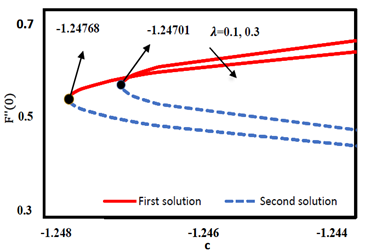
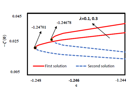
, and there is no solution for ![]() The critical point
The critical point ![]() for
for ![]() and 0.3 are
and 0.3 are ![]() 1.24701 and
1.24701 and ![]() 1.24768 (see Figures. 1-2). The solution domain expands with increasing
1.24768 (see Figures. 1-2). The solution domain expands with increasing
![]() , and
, and ![]() is
more negative for the non-Newtonian case than the Newtonian case, highlighting
that
is
more negative for the non-Newtonian case than the Newtonian case, highlighting
that ![]() plays a significant role in the existence of solutions, as supported
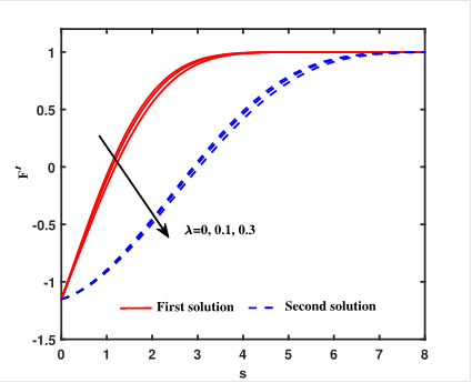
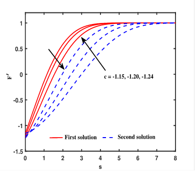
by theoretical results. Figure. 3 demonstrates a significant decrease in the
velocity profile
plays a significant role in the existence of solutions, as supported
by theoretical results. Figure. 3 demonstrates a significant decrease in the
velocity profile![]() with increasing
with increasing ![]() for both
solution branches. It is observed that the thickness of the momentum boundary
layer is larger for Newtonian fluid than for non-Newtonian fluid.
for both
solution branches. It is observed that the thickness of the momentum boundary
layer is larger for Newtonian fluid than for non-Newtonian fluid.
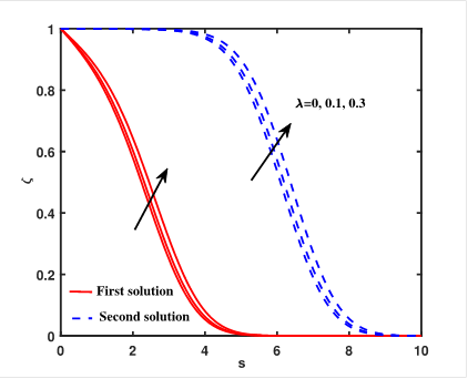
The
temperature profile for both solutions increases with the non-Newtonian
parameter ![]() (see Figure.
4), resulting in a rise in the thickness of the thermal boundary layer. Figure.
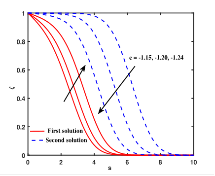
5 shows that
(see Figure.
4), resulting in a rise in the thickness of the thermal boundary layer. Figure.
5 shows that ![]() decreases in the first solution but increases in
the second solution as
decreases in the first solution but increases in
the second solution as ![]() increases. Conversely,
increases. Conversely, ![]() increases with
increases with ![]() in
the first
solution while decreasing in the second solution (see Figure. 6). The momentum
and thermal boundary layer thicknesses are found to be smaller in the first
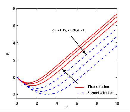
solution compared to the second solution. In Figure. 7,
in
the first
solution while decreasing in the second solution (see Figure. 6). The momentum
and thermal boundary layer thicknesses are found to be smaller in the first
solution compared to the second solution. In Figure. 7, ![]() decreases in the first solution but increases in
the second solution as
decreases in the first solution but increases in
the second solution as ![]() increases. Initially, each curve shows a decline,
reaching certain negative values for small
increases. Initially, each curve shows a decline,
reaching certain negative values for small ![]() . However,
these values gradually increase and become positive beyond a certain distance
from the sheet.
. However,
these values gradually increase and become positive beyond a certain distance
from the sheet.
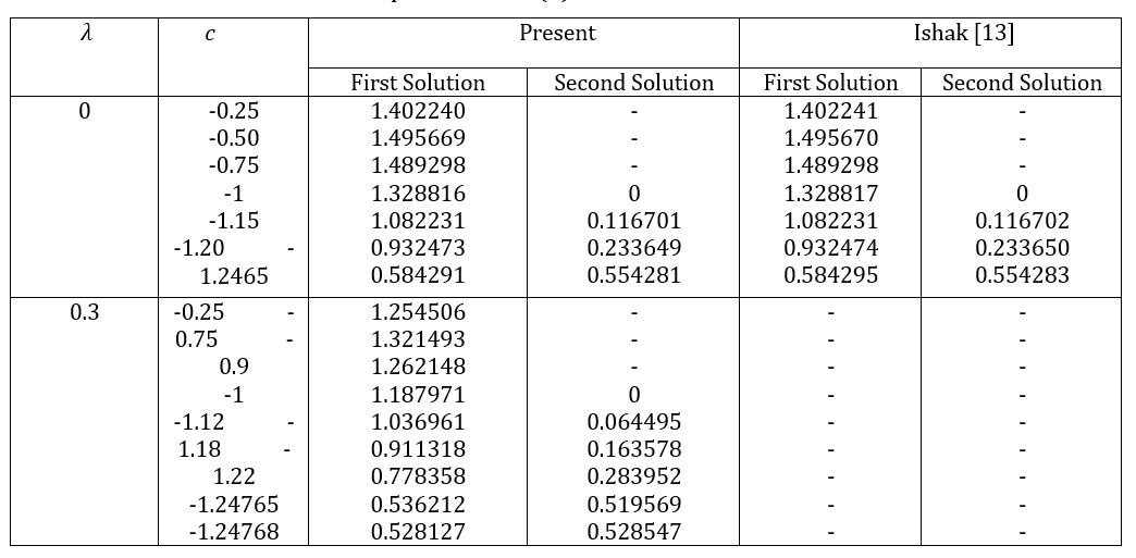
Table 3:Smallest eigenvalues for different
|
First solution |
Second solution |
||
|
0.1 |
-1.24 -1.19 -1.18 |
0.157272 0.573241 0.627739 |
-0.258123 -0.598794 -0.638914
|
|
0.3 |
-1.24 -1.21 -1.20 |
0.016590 0.341042 0.405736 |
-0.348644 -0.571240 -0.618171
|
The stability analysis is performed using the BVP4C function in MATLAB software. The detailed procedure and calculation are mentioned in Appendix A. As shown in Table 3, the smallest eigenvalues for both solutions are computed for different shrinking parameters c. In the first solution, the eigenvalues are observed to be real and positive, while in the second solution, they are negative. Because of the positive smallest eigenvalues, initial disturbances in the fluid
flow diminishes over time,
that is ![]() as ϵ → ∞. Consequently, the first solutions are
determined to be stable. However, the smallest negative eigenvalue suggests an
amplification of initial disturbances in the flow, given by
as ϵ → ∞. Consequently, the first solutions are
determined to be stable. However, the smallest negative eigenvalue suggests an
amplification of initial disturbances in the flow, given by ![]() indicating that the flow solutions (second
solution) exhibit unstable behavior. The stable solution is physically
meaningful for the above flow, whereas the unstable solution is not.
indicating that the flow solutions (second
solution) exhibit unstable behavior. The stable solution is physically
meaningful for the above flow, whereas the unstable solution is not.
7 Conclusion
The research delved into the boundary layer stagnation-point flow and convective heat transfer on a linearly stretching/shrinking surface in non-Newtonian Williamson fluid. A suitable similarity transformation is employed to convert the PDEs into nonlinear ODEs for modelling purposes. The application of the shooting method illustrates the existence of a solution and examines its characteristics. The numerical solution for this study is acquired by implementing the shooting-based numerical code in MATLAB, specifically using the BVP4C solver. Further, a connection between theoretical results and numerical investigation has been made. A temporal stability analysis is carried out to identify a stable solution, providing insights into the primary flow dynamics. The main findings of this study can be outlined as follows
- The existence of a unique solution to the nonlinear equation is proved for the stretching/shrinking parameter c∈(-1,∞).
- Dual solutions exist for c ∈ [c_T,-1], and there does not exist any solution for c∈(-∞,c_T ).
- The velocity profile F'(s) decreases with non-Newtonian parameter λ in both solution branches, whereas the temperature profile ζ(s) increases with λ.
- In the first solution branch, the boundary layer thickness (for both momentum and thermal) is smaller compared to the second solution branch. Additionally, the solution domain expands with increasing λ.
- Stability analysis indicates that the first solution branch is physically acceptable, as all the smallest eigenvalues are positive, whereas the second solution branch is unstable.
- An asymptotic solution for large c>0 shows that the expressions F''(0)~-1.316134 c^(3\/2) and ζ^' (0) ~ -0.556919 c^(1\/2) as c →∞.
Appendix A
A study on temporal stability is carried out using the foundational research of Merkin [16], who indicated potential practical unreliability in the lower branch. To achieve this, we take into account the time-varying representation of equations (11)-(12)
![]()
![]() ,
,
![]()
Due to the presence of a time variable, we introduce the following new dimensionless variable
 (A2)
(A2)
Here, ![]() represents the
updated non-dimensional time parameter. Employing
represents the
updated non-dimensional time parameter. Employing ![]() refers to an
initial value challenge, raising the query of which solution holds physical
validity. By using (A2), from (A1), we get
refers to an
initial value challenge, raising the query of which solution holds physical
validity. By using (A2), from (A1), we get
![]()
where, ![]() denotes the
derivative concerning
denotes the
derivative concerning ![]() and superscript
and superscript ![]() represents
derivative with respect to
represents
derivative with respect to ![]() . The boundary
conditions for the above time dependent flow are
. The boundary
conditions for the above time dependent flow are
![]() (A4)
(A4)
To assess the stability of
the steady flow solution, ![]() and
and ![]() satisfy equations (11)-(12), a group of perturbed
equations is examined to facilitate the separation of variables
satisfy equations (11)-(12), a group of perturbed
equations is examined to facilitate the separation of variables
![]()
![]() (A5)
(A5)
Here, ![]() is an unknown eigenvalue, and both
is an unknown eigenvalue, and both ![]() and
and ![]() are significantly smaller than
are significantly smaller than ![]() and
and ![]() . Solving the eigenvalue problem (A4)-(A5)
provides a series of eigenvalues
. Solving the eigenvalue problem (A4)-(A5)
provides a series of eigenvalues ![]() . If
. If ![]() is negative, it implies initial disturbance
growth, indicating flow instability. Conversely, when
is negative, it implies initial disturbance
growth, indicating flow instability. Conversely, when ![]() is positive, there is initial decay, signifying
flow stability. Substituting (A5) into (A3)-(A4) and leads to the following
linearized problem
is positive, there is initial decay, signifying
flow stability. Substituting (A5) into (A3)-(A4) and leads to the following
linearized problem
![]()
![]() ,
,
![]()
![]() ,
,
![]() (A6)
(A6)
Now, we are putting ![]() for check the stability of steady state solution
and considering
for check the stability of steady state solution
and considering ![]() and
and ![]() , then equations (A6) become
, then equations (A6) become
![]()
![]() ,
,
![]() ,
,
![]()
![]() (A7)
(A7)
Solving equations (A7) numerically, one can easily get the smallest eigenvalue. See [24]
for a detailed explanation for determining the smallest eigenvalue. To solve
it, we need an additional boundary condition. Therefore, without loss of
generality, we take ![]() .
.
References
[1] Chhabra R P (2010) non-Newtonian fluids: an introduction. Rheology of complex fluids pp.3-34. View Article
[2] Irgens F (2014) Rheology and non-Newtonian fluids, vol. 190 Springer. View Article
[3] Williamson R V (1929) The flow of pseudoplastic materials. Industrial & Engineering Chemistry 21(11), 1108-1111. View Article
[4] Lyubimov D, Perminov A (2002) Motion of a thin oblique layer of a pseudoplastic fluid. Journal of Engineering Physics and Thermophysics 75(4), 920-924. View Article
[5] Nadeem S, Ashiq S and Ali M (2012) Williamson fluid model for the peristaltic flow of chyme in small intestine. Mathematical Problems in Engineering. View Article
[6] Akbar N S (2015) Mixed convection analysis for blood flow through arteries on Williamson fluid model. International Journal of Biomathematics 8(04), 1550045. View Article
[7] Khan N A, Khan H (2014) A boundary layer flows of non-Newtonian Williamson fluid. Nonlinear Engineering 3(2), 107-115. View Article
[8] Nadeem S, Hussain S (2014) Heat transfer analysis of Williamson fluid over exponentially stretching surface. Applied Mathematics and Mechanics 35(4), 489-502. View Article
[9] Hamid A, Khan M and Khan U (2018) Thermal radiation effects on Williamson fluid flow due to an expanding/contracting cylinder with nanomaterials: dual solutions. Physics Letters A 382(30), 1982-1991. View Article
[10] Paullet J, Weidman P (2007) Analysis of stagnation point flow toward a stretching sheet. International Journal of Non-Linear Mechanics 42(9), 1084-1091. View Article
[11] Wang C (2008) Stagnation flow towards a shrinking sheet. International Journal of Nonlinear Mechanics 43(5), 377-382. View Article
[12] Crane L J (1970) Flow past a stretching plate. Zeitschrift f"ur angewandte Mathematik und Physik ZAMP 21, 645-647. View Article
[13] Ishak A, Lok Y Y and Pop I (2010) Stagnation point flow over a shrinking sheet in a micropolar fluid. Chemical Engineering Communications 197(11), 1417-1427. View Article
[14] Sarkar G M, Sahoo B (2020) Dual solutions of magnetohydrodynamic boundary layer flow and a linear temporal stability analysis. Proceedings of the Institution of Mechanical Engineers, Part E: Journal of Process Mechanical Engineering 234(6), 553-561. View Article
[15] Haq R U, Zahoor Z and Shah S S (2023) Existence of dual solution for MHD boundary layer flow over a stretching/shrinking surface in the presence of thermal radiation and porous media: KKL nanofluid model. Heliyon 9(11). View Article
[16] Merkin J (1986) On dual solutions occurring in mixed convection in a porous medium. Journal of engineering Mathematics 20(2), 171-179. View Article
[17] Roy N C, Pop I (2023) Dual solutions of a nanofluid flow past a convectively heated nonlinearly shrinking sheet. Chinese Journal of Physics 82, 31-40. View Article
[18] Usafzai W K, Pop I and Revnic C (2024) Dual solutions for the two-dimension copper oxide with silver (CuO-Ag) and zinc oxide with silver (Zno-Ag) hybrid nanofluid flow past a permeable shrinking sheet in a dusty fluid with velocity slip. International Journal of Numerical Methods for Heat & Fluid Flow 34(1), 259-279. View Article
[19] Miklavcic M, Wang C (2006) Viscous flow due to a shrinking sheet. Quarterly of Applied Mathematics 64(2), 283-290. View Article
[20] Van Gorder R A, Vajravelu K and Pop I (2012) Hydromagnetic stagnation point flow of a viscous fluid over a stretching or shrinking sheet. Meccanica 47(1), 31-50. View Article
[21] Sarkar G M, Sarkar S and Sahoo B (2022) Analysis of Hiemenz flow of Reiner-Rivlin fluid over a stretching/shrinking sheet. World Journal of Engineering 19(4), 522-531. View Article
[22] Abdal S, Hussain S, Siddique I, Ahmadian A and Ferrara M (2021) On solution existence of MHD Casson nanofluid transportation across an extending cylinder through porous media and evaluation of priori bounds. Scientific Reports 11(1), 7799. View Article
[23] Mondal, D., Pandey, A. K., & Das, A. (2025). Flow and heat transfer analysis of an ionanofluid above a rotating disk undergoing torsion. Chinese Journal of Physics, 93, 127-157. View Article
[24] Mondal, D., Das, A., & Pandey, A. K. (2025). Existence and nonuniqueness of solutions for flow driven by a revolving hybrid nanofluid above a stationary disk. Journal of Mathematical Analysis and Applications, 129743 View Article