Journal of Fluid Flow, Heat and Mass Transfer (JFFHMT)
ISSN: 2368-6111

Volume 12 - Year 2025 - Pages 352-363
DOI: 10.11159/jffhmt.2025.034
Pressure Tooling Problem with Thermal Condition for Non-Newtonian Fluid
Nawalax Thongjub 1, Supachara Kongnuan1
1Thammasat University, Department of Mathematics and Statistics,
Faculty of Science and Technology, Pathumthani, Thailand, 12120
nawalax@mathstat.sci.tu.ac.th; supachara@mathstat.sci.tu.ac.th
Abstract - This study investigates pressure tooling issues in Non-Newtonian fluids under both isothermal and non-isothermal conditions, focusing on annular drag flow. The analysis considers creeping pressure tooling flow in a two-dimensional axisymmetric cylindrical coordinate system. These problems are modeled using non-linear partial differential equations derived from the Navier–Stokes, heat transfer, and Oldroyd-B formulations. To solve the governing and constitutive equations, the Semi-implicit Taylor–Galerkin pressure-correction finite element method (STGFEM) is employed. For polymer melt flows at Weissenberg numbers (We), a feedback mechanism is introduced to adjust the inlet boundary conditions. To enhance convergence, the streamline-upwind/Petrov–Galerkin approach is incorporated. Finally, the swelling ratio of the extruded product is compared with experimental data from pressure tooling applications. The computed extrudate dimensions show strong agreement with experimental results and reasonable consistency with analytical predictions. While experimental and numerical outcomes are closely matched, a discrepancy is observed when compared to the analytical model. As a result, non-isothermal systems exhibit greater pressure drop, shear rate, and elongation compared to isothermal cases. Thermal effects weaken the intermolecular bonding in polymers, thereby influencing shear rate and pressure drop. The temperature of pressure-tooling process is very useful to keep the polymeric material from hardening and to support it easier to propel the polymer stream through the die. The maximum temperature is observed at the leading edge of the pressure-tooling domain, after which it decreases progressively and eventually diminishes once the wire becomes coated with the polymer melt in the free-surface region.
Keywords: Isothermal condition, Non-isothermal conditions, Pressure tooling
© Copyright 2025 Authors - This is an Open Access article published under the Creative Commons Attribution License terms Creative Commons Attribution License terms. Unrestricted use, distribution, and reproduction in any medium are permitted, provided the original work is properly cited.
Date Received: 2025-05-18
Date Revised: 2025-09-17
Date Accepted: 2025-09-30
Date Published: 2025-10-18
1. Introduction
Nowadays, a lot of polymer products such as PVC pipes, electric wires, fiber optics and plastic bags are produced to support consumers. After the time has passed for a long period, a lot of polymer materials are used up so many factories tried to find out new plastic compounds for substitution. The real experiments were set up to check the quality of the outcome so the process is time-consuming and costly due to the trial and error tests. In order to save money and cut time, the simulations of real problems are created with mathematical models so the solution is achieved by numerical methods. Since all models approaching to real world are complicated, the simplest expression is started for Newtonain fluid before developing to complex flow. In case of polymer melts, the fluid is viscoelastic so the behavior of flow can explain with stress equations such as power law, Maxwell and Oldroyd-B models. The constitutive model of Oldroyd-B fluid is proposed to represent the high-density polyethylene that is popularly used in the manufacture of plastics. For the coating processes, the polymeric beads are melted under heat while they are passing with friction along the extrusion screw. Under this research, the wire coating flow for annular pressure tooling die is considered with cylindrical coordinate system that is suitable to specifying geographic position.
This research is focused on thermal condition of annular flow for the Newtonian and Oldroyd-B fluids using three different geometries; namely, stick-slip, die-swell and pressure tooling domains under isothermal and non-isothermal conditions. These problems are solved by a semi-implicit Taylor-Galerkin pressure-correction finite element method (STGFEM) [1] with feedback boundary scheme [2] based on two-dimensional system. For the stick-slip and die-swell phenomenon [3], the materials of polymer melt show steep shear stress and strong elongation when the flow contracts at die exit section then the streamline path of viscoelastic fluid suddenly changes direction from stick to slip boundary, so the trajectory is swell at the surface because this region has high pressure to push the fluid flow pass die. For the thermal condition, the initial value at inlet is the major boundary to set for solving the solution in domain but the calculation would be terminated when the program tries to run with high Weissenberg number. Actually, the calculation of Oldroyd-B model has confronted to breakdown with infinite error after the machine keeps trying to rerun high Weissenberg number.
The stick-slip problem [4] is the simulation case for specific condition that is not actual occurrence whilst the die-swell in the extrusion process approaches real problem more than stick-slip case. This process is applied to pharmaceutical manufacturing [5,6], PVC pipe factory and wire cable industry. For the extrusion process, the high speed near die exit makes the violent shear stress at die wall and then the high swelling ratio appears. The surface of extrudate is confronted with sharp skin when viscoelastic fluid moves pass die with high velocity, so it leads to severe crack which is the defect of the products.
In extrusion process, the free surface method was solved by integral transforms for adjusting the stick-slip shape then move on to free surface geometry. The flow passes a stick region in die wall and swell after die then the conflict of two regions makes the singular point for a severe shear stress and steep velocity gradients. The singularity point was measured by capillary viscometer in polystyrene fluid [7]. This research described the effect of molecular weights on swelling ratio and the swell surface is almost dependent on the aspect ratio L/D (length/diameter). The singularity effect [8] of stress and strain is reduced by semi-radial singularity mapping theory but this theory is not widespread because there is a scope of use with some liquids.
The models of non-Newtonian flow such as the Oldroyd-B and Phan-Thien/Tanner fluids are represented by the Navier-Stokes equations that express the state of flow whilst the mathematical model of viscoelastic problem is a form of non-linear partial differential equations under conservation law of mass and momentum. Since all mathematical models are non-linear partial differential equations then the analytical solution is hard to find.
To avoid testing from trial, the approximate solution is used alternatively with high-performance computing, so the time is cut off and the budget is saved. For the numerical method, the procedure is easy to modify the characteristics of parameter when the boundary condition is changed. At first, the wire-coating simulation with the simple constitutive model of viscoelastic flow, that is power-law fluid, is solved by finite element method under the isothermal condition [9] but the solution does not get along well with real experiment and then the influence of the temperature boundary condition is investigated [10].
Then the slip condition was added in the wire-coating flow of Newtonian and power-law fluids at the solid boundaries [11]. Furthermore, a wire-coating flow of a low-density polyethelene (LDPE) was represented by power-law fluids under thermal and isothermal cases via the finite element method with SUPG scheme [12] and this numerical result was close to the experiment. The various numerical schemes were developed to solve a wire-coating problem with a viscoelastic flow. A tube-tooling die in a non-isothermal case was solved by couple and decouple methods [13]. A tube-tooling of wire-coating flow with Phan-Thien/Tanner constitutive model (PTT) [14,15,16] and then the contraction point of wire-coating was calculated for Phan-Thien/Tanner model with tube-tooling flow [17,18]. For Oldroyd-B fluid, this research has shown the effect of the slip in 4:1 contraction flow through which the slip can reduce the stress and vortex at sharp corner [19].
The literature reviews of extrudate swell flows under heat condition were explained as follows: The White-Metzner constitutive model [20] for non-isothermal case was solved by finite element method. The simulation of the extrusion for viscoelastic fluid under heat condition was described with a K-BKZ equation [21]. The temperature of wire coating process is measured in screw extruder when it is rotated within the barrel from the effect of shear heating of polymer. The cable-coating extrusions were simulated at the isothermal system whilst the experiment has indicated that thermal is dominant effect to viscosity and pressure. The numerical research under temperature [22,23] matches well with experimental results with non-isothermal condition. For more deeply detail to nanofluid scale, the heat transfer characteristics in a double-pipe counter-flow have been investigated under the finite volume scheme [24].
To study the effect of temperature between annular die-swell and pressure-tooling flows, the mathematical models via the Navier-Stokes equations and Oldroyd-B model under thermal condition are proposed. The governing equations have been solved by finite element method with Taylor-Galerkin pressure-correction scheme to describe the annular die-swell flow passing the entrance. After flow developed to die exit, the stream trajectory behaves as free surface in a two-dimensional domain. The various Weisenberg numbers are represented for the different flow behaviors as shown in terms of the velocities, stresses, pressure and temperature. The local velocity gradient recovery scheme and streamline-upwind/Petrov-Galerkin method are employed to improve the stability of the solution.
2. Materials and Governing Equations
2.1 Non-Newtonian Fluid
The velocity divergence of creeping motion for incompressible fluid, whose density does not vary, under the principle of conservation of mass is shown as the continuity equation as Eq. 1. The dimensionless Navier-Stokes momentum equation without gravity appears in Eq. 2. Both equations are useful to describe the physical motion of stream path including density (ρ), pressure (p
),
extra-stress tensor (![]() ) and time (t).
) and time (t).
|
|
(1) |
![]() (2)
(2)
where ![]() is
the non-dimensional Reynolds number and
is
the non-dimensional Reynolds number and ![]() that
is a ratio of the inertial to viscous forces,
that
is a ratio of the inertial to viscous forces, ![]() is
characteristic velocity,
is
characteristic velocity, ![]() is characteristic length,
is characteristic length, ![]() is the
zero-shear viscosity and
is the
zero-shear viscosity and![]() ,
, ![]() is the
polymeric viscosity and
is the
polymeric viscosity and ![]() is the
solvent viscosity. The flow behavior depends on shear models
is the
solvent viscosity. The flow behavior depends on shear models ![]() and
and  where
the extra-stress tensor is combination of stress tensor (
where
the extra-stress tensor is combination of stress tensor (![]() ) and the rate
of deformation tensor (
) and the rate
of deformation tensor (![]() ).
).
The Oldroyd-B constitutive model consists of non-dimensionless equation as Eq. 3.
![]() (3)
(3)
where ![]() is the
non-dimensional Weisenberg number.
is the
non-dimensional Weisenberg number. ![]() and
and ![]() is the
relaxation time.
is the
relaxation time.
2.2 Thermal flow
For incompressible non-isothermal flow, the conservation of energy is used to discuss the effect of shear viscosity and temperature. The non-dimensional conservation of energy is represented in Eq. (4).
![]() (4)
(4)
where ![]() is
temperature and
is
temperature and ![]() is the non-dimensional thermal
Peclect number and
is the non-dimensional thermal
Peclect number and ![]() , c is specific heat,
and
, c is specific heat,
and ![]() is
thermal conductivity, and
is
thermal conductivity, and ![]() is the heat source. The
zero-shear viscosity for viscous fluid under heat is
is the heat source. The
zero-shear viscosity for viscous fluid under heat is ![]() where
where
![]() is
the temperature at the end of pug flow, and
is
the temperature at the end of pug flow, and ![]() is the
material constant for polymeric melt. In this research,
is the
material constant for polymeric melt. In this research, ![]() for
high-density polyethylene (HDPE).
for
high-density polyethylene (HDPE).
3. Numerical Methods
The fractional steps are split to 3 stages for converting the non-linear differential form to the system of linear equations before the computation of the finite element method (FEM) is calculated to estimate the solution.
3.1 Semi-implicit Taylor-Galerkin pressure-correction finite element method
The semi-implicit Taylor-Galerkin pressure-correction finite element method split Navier-stokes Eq. 2 to the three fractional stages per time step but the Oldroyd-B and temperature models are discritized to the half time step and full time step. The first and last steps are solved for the velocities but the middle step is calculated for the pressure variable.
Step 1a: The half time step of velocities, temperature and stresses can be derived from the equations below:
![]() (5)
(5)
 (6)
(6)
![]() (7)
(7)
Step 1b: The transient stage of intermediate velocities, temperature and stresses is updated as in the following equations.
![]() (8)
(8)
 (9)
(9)
![]() (10)
(10)
Step 2: Full time step of pressure is related to intermediate velocity according to the equation.
![]() (11)
(11)
Step 3: The full time step velocities is expressed as:
![]() (12)
(12)
3.2 Feedback of pressure-driven velocity flow
The
feedback of this procedure is an occurrence that appears when the outcome of
velocity and pressure from each time step is used as input back into the inlet
boundary condition as part of a chain to present for accelerating the
convergent iterative procedures of solving the system of linear equations. The
solution is duplicated for upstream section at the same vertical nodes in the
stabilized column and return values back to inlet boundary. For example, in
Figure 1 the possible column can be nodes in C2 (column 2), C3, C4 and C5 and
if the C3 is chosen then the values of velocity and pressure of nodes 9, 10, 11
and 12 will be the initial condition for nodes 1, 2, 3 and 4, respectively.
Firstly, the difference of time step is set up at ![]() as the
rate of error. After the feedback of the pressure-driven velocity flow is
inserted, the difference of time and error is reduced gradually to prevent the
diverging circumstance. This cycle is operated until the inlet boundary
maintains the stability and the converged solution is obtained.
as the
rate of error. After the feedback of the pressure-driven velocity flow is
inserted, the difference of time and error is reduced gradually to prevent the
diverging circumstance. This cycle is operated until the inlet boundary
maintains the stability and the converged solution is obtained.
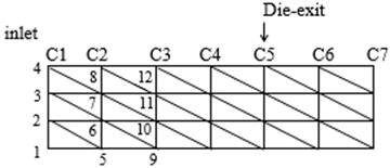
Figure 1. Example of mesh geometry.
For die-swell flow, the location of free surface over die is calculated from the solution of stick-slip case as Figure 2 and the body of extrudate section is represented in Figure 3. The distance from symmetry line to top free jet be called swelling ratio as defined by Eq. 13 and is the combination of die radius and the fraction between radial velocity to axial velocity.
 (13)
(13)
where r
is radial position, z is axial position, R is die radius, ![]() is radial velocity and
is radial velocity and ![]() is axial velocity.
is axial velocity.
4. Problem Specification
There are three different geometrical domains, that are stick-slip, die swell and pressure-tooling shapes. At first domain of stick-slip body is set up to run in a program as a simple case. The die-swell case is produced from short die but the pressure-tooling form is received from long die.
4.1 Stick-slip flow
The stick-slip domain as seen in Figure 2, consists of two zones with different boundary conditions, in die area and over die area. The stick boundary condition is applied at die wall while the slip boundary condition is concerned at free jet section. The stick-slip mesh is divided to 1,944 triangular elements and 4,033 nodes. The radial and axial velocities vanish at die boundary and both velocities are calculated on the free surface.
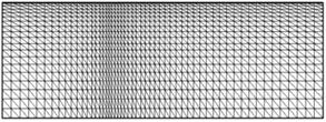
Figure 2. Mesh geometry of stick-slip flow.
4.2 Die-swell flow
First, the stick-slip problem is simulated to get the converge result and then move on to compute the die-swell flow by taking the solution of stick-slip case to start at initial condition. Consequently, the swelling ratio represented in Eq. 13 is evaluated to adjust free surface geometries. The adaptive die-swell mesh is shown in Figure 3. The thermal condition is added to study the behavior of the velocity, stresses and pressure for die-swell flow via Oldroyd-B constitutive model. The boundary conditions are detailed in Figure 4 as same inlet condition as pressure-tooling issue.
Figure 3. Mesh geometry of die-slip flow.
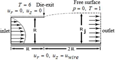
Figure 4. Die-swell thermal flow.
At the inlet, the boundary conditions for the annular flow are set as following equations.
![]()
 (14)
(14)
The condition at the end is plug flow for all problems with following equations.
![]() (15)
(15)
4.3 Pressure-tooling flow
The structure of the pressure-tooling problem shown in Figure 5 is discretized into a mesh consisting of 3,810 triangular elements, 7,905 nodes, and 17,858 degrees of freedom. According to the study in [25], mesh convergence was systematically evaluated, ensuring that the computational domain remains unaffected by artifacts and thus provides reliable results. The polymer bulk is extruded from the screw with wire speed according to the bottom boundary. The detail of specific boundary conditions is described in Figure 6.
Figure 5. Mesh geometry of pressure-tooling flow.
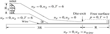
Figure 6. Pressure-tooling flow.
5. Results and Discussion
5.1 Result of Stick-slip
The result of the stick-slip contour
color solution is plotted for ![]() and
and ![]() as shown in
Figure 7. The radial velocity for all Weissenberg numbers approaches zero as
seen in Figure 7(a). The axial velocity is annular flow at the inlet and the
maximum value is located at symmetry line as shown in Figure 7(b). When the
stick-slip flow develops to plug flow at the end of downstream, the pressure is
maximized at the entrance and gradually decreases until zero at the outlet as
depicted in Figure 7(c). The maximum value of
as shown in
Figure 7. The radial velocity for all Weissenberg numbers approaches zero as
seen in Figure 7(a). The axial velocity is annular flow at the inlet and the
maximum value is located at symmetry line as shown in Figure 7(b). When the
stick-slip flow develops to plug flow at the end of downstream, the pressure is
maximized at the entrance and gradually decreases until zero at the outlet as
depicted in Figure 7(c). The maximum value of ![]() ,
, ![]() , and
, and ![]() at die
exit are displayed in Figure 7(d), 7(e) and 7(f), respectively. The peak value
of
at die
exit are displayed in Figure 7(d), 7(e) and 7(f), respectively. The peak value
of ![]() appears at swell area near die exit as
detailed in Figure 7(g). Figure 7(h) shows maximum value of the temperature at
inlet which then gradually decreases to 1 at the outlet.
appears at swell area near die exit as
detailed in Figure 7(g). Figure 7(h) shows maximum value of the temperature at
inlet which then gradually decreases to 1 at the outlet.
(a)
![]()
(b)
![]()
(c)
![]()
(d)
![]()
(e)
![]()
(f)
![]()
(g)
![]()
(h)
![]()
Figure 7. Stick-slip for Oldroyd-B fluid at ![]() .
.
5.2 Result of Die-swell
Die-swell flow
of Oldroyd-B fluid is developed from the domain of stick-slip problem and the
contour color result of extrudate swell for ![]() and
and ![]() is shown in
Figure 8(a)-8(h). The exhibition of color contour plots for the radial
velocity, axial velocity, pressure,
is shown in
Figure 8(a)-8(h). The exhibition of color contour plots for the radial
velocity, axial velocity, pressure, ![]() ,
, ![]() ,
, ![]() ,
, ![]() and temperature of swell effect are very
similar to those in stick-slip model. Because of size enlargement phenomenon
makes the height of radial direction after die growth up so the radial
velocity,
and temperature of swell effect are very
similar to those in stick-slip model. Because of size enlargement phenomenon
makes the height of radial direction after die growth up so the radial
velocity, ![]() ,
, ![]() and
and ![]() are higher than those corresponding to
stick-slip but it is converted for the axial velocity, pressure and
are higher than those corresponding to
stick-slip but it is converted for the axial velocity, pressure and ![]() .
.
(a)
![]()
(b)
![]()
(c)
![]()
(d)
![]()
(e)
![]()
(f)
![]()
(g)
![]()
(h)
![]()
Figure 8. Die-swell for Oldroyd-B fluid at ![]() .
.
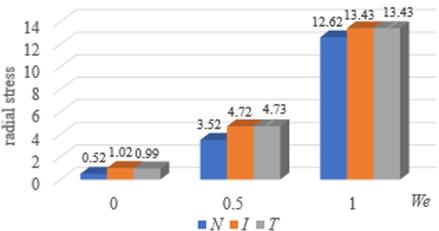
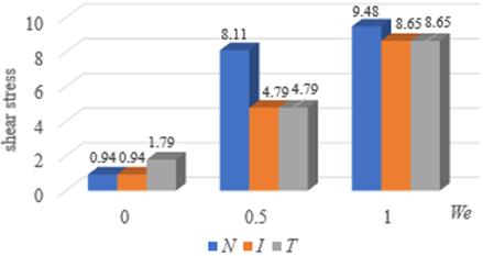
For die-swell flow, the parameters of
pressure drop ![]() ,
shear stress
,
shear stress ![]() and stress in direction
and stress in direction ![]()
![]() , and in direction
, and in direction ![]()
![]() are compared with the result from
reference [25] under non-thermal effect (N) and the outcome of this work
for isothermal (I) and thermal conditions (T). The round brackets
containing parameter with subscripts N, I or T as symbols
are compared with the result from
reference [25] under non-thermal effect (N) and the outcome of this work
for isothermal (I) and thermal conditions (T). The round brackets
containing parameter with subscripts N, I or T as symbols ![]() ,
, ![]() and
and ![]() indicate the value of those parameter for
the non-thermal effect, isothermal and thermal conditions, respectively.
indicate the value of those parameter for
the non-thermal effect, isothermal and thermal conditions, respectively.
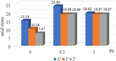
Table 1 shows the comparison of
die-swell flow for Newtonian and Oldroyd-B fluid between non-thermal,
isothermal and non-isothermal processes. The viscosity and elongation are
greatly proportional to Weissenberg number the same as pressure drop and
stresses. Another dominant effect to pressure drop is heat conduction but it
gives a little significance for ![]() ,
, ![]() and
and ![]() . The
stresses
. The
stresses ![]() and
and ![]() slightly
drop when Weissenberg number is 1 conversely to stress
slightly
drop when Weissenberg number is 1 conversely to stress ![]() .
.
Table 1. The comparison of die-swell flow for Oldroyd-B fluid between non-thermal, isothermal and non-isothermal conditions.
|
We |
0 |
0.5 |
1 |
|
|
4.94 |
14.53 |
32.92 |
|
|
4.86 |
17.34 |
37.59 |
|
|
18.18 |
17.76 |
38.26 |
|
|
0.94 |
8.11 |
9.48 |
|
|
0.94 |
4.79 |
8.65 |
|
|
1.79 |
4.79 |
8.65 |
|
|
15.14 |
23.84 |
19.62 |
|
|
10.24 |
18.99 |
18.97 |
|
|
7.47 |
18.99 |
18.97 |
|
|
0.52 |
3.52 |
12.62 |
|
|
1.02 |
4.72 |
13.43 |
|
|
0.99 |
4.73 |
13.43 |
(a)
![]()
(b)
![]()
(c)
![]()
(d)
![]()
Figure 9. The bar charts of die-swell flow for Oldroyd-B fluid.
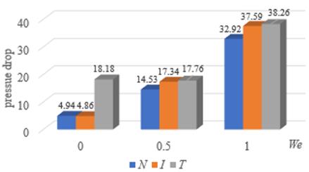
The whole data of table 1 are pick up to draw bar charts as details in Figure 9. Figure 9(a)-9(d) are compared under non-thermal isothermal and non-isothermal systems with four-character values of pressure drops, shear, radial and axial stresses, respectively. The radial and axial stresses are slightly different when We equals 1. Heat shows the dominant effect for Newtonian flow while isothermal and non-isothermal system give almost the same values for Oldroyd-B fluid.
5.3 Result of Pressure-Tooling Flow
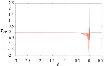
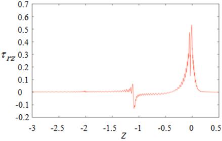
At first of the simulation for the
pressure tooling problem with annular die, the appropriate value of ![]() is 0.88 for
Oldroyd-B fluid and the high
is 0.88 for
Oldroyd-B fluid and the high ![]() is chosen to run for difficult
flow. On top edge region, the value of shear stress starts oscillating as seen
in Figure 10 from z direction at the point -1.50 to 0.50 and the peak is
1.98 near die exit
is chosen to run for difficult
flow. On top edge region, the value of shear stress starts oscillating as seen
in Figure 10 from z direction at the point -1.50 to 0.50 and the peak is
1.98 near die exit ![]() as similarly to the result
along bottom line, that generates two waves, the small peak of 0.05 at
as similarly to the result
along bottom line, that generates two waves, the small peak of 0.05 at ![]() and the big
apex of 0.54 at die outlet.
and the big
apex of 0.54 at die outlet.
For Figure 11, the extreme point of axial stress at top edge is 6.69 whilst the maximal value at the bottom is 0.80 and the small peak appears at the second acute corner where it contacts with wire. As stated above, the shear rate of Newtonian and viscoelastic fluids between isothermal and non-isothermal condition are compared in Figure 12. The shear rate at the top edge jumps to maximum value near die exit due to contraction point where the fluid is pushed out from mold made the free surface swell. At the top edge, the peaks of shear rate for isothermal and non-isothermal happen near die exit with maximum values of 606.41 and 649.46, respectively but the bottom edge created twice peaks at contraction point and die exit.
(a) At top edge
(b) At bottom edge
Figure 10. ![]() for
isothermal condition.
for
isothermal condition.
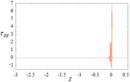
(a) At top edge
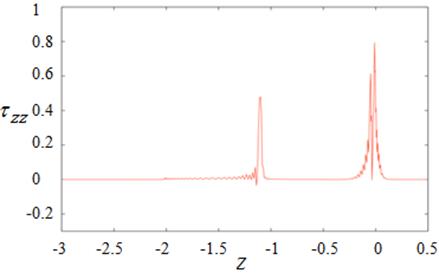
(b) At bottom edge
Figure 11. ![]() for isothermal condition.
for isothermal condition.
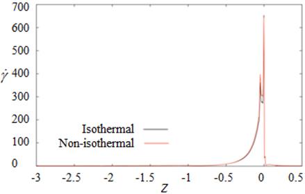
(a) At top edge
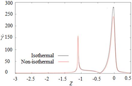
(b) At bottom edge
Figure 12. ![]() for
isothermal
for
isothermal
Table 2. The comparison of pressure-tooling flow for Oldroyd-B fluid between isothermal and non-isothermal condition.
|
We |
0.5 |
1 |
1.5 |
2 |
|
|
1.08 |
1.07 |
1.07 |
1.07 |
|
|
1.08 |
1.07 |
1.07 |
1.07 |
|
|
3.45 |
3.45 |
3.45 |
3.45 |
|
|
3.41 |
3.41 |
3.42 |
3.42 |
|
|
3.21 |
1.65 |
1.12 |
0.83 |
|
|
3.25 |
1.66 |
1.12 |
0.84 |
|
|
8.28 |
3.98 |
2.61 |
1.94 |
|
|
8.49 |
4.07 |
2.67 |
1.98 |
|
|
26.13 |
13.18 |
8.81 |
6.61 |
|
|
26.46 |
13.33 |
8.91 |
6.69 |
|
|
0.13 |
0.07 |
0.05 |
0.03 |
|
|
0.13 |
0.07 |
0.05 |
0.03 |
|
|
609.81 |
607.22 |
606.64 |
606.41 |
|
|
656.81 |
651.62 |
650.10 |
649.46 |
|
|
11.06 |
8.41 |
7.40 |
7.40 |
|
|
11.42 |
8.82 |
7.73 |
7.71 |
|
|
132.09 |
126.90 |
125.15 |
124.27 |
|
|
1019.80 |
980.33 |
967.00 |
960.31 |
From Table 2, the heat does not affect
velocities but it is significant to pressure and
stresses. All stresses ![]() , the pressure drop
, the pressure drop ![]() , the shear rate
, the shear rate ![]() and the elongation rate
and the elongation rate ![]() are reduced when Weissenberg
number increases. Under non-isothermal system, the pressure drop is 6.73 times
greater than that of isothermal system. The shear rate and elongation rate of
non-isothermal case are 7% and 4% of the values for isothermal stage,
respectively. The heat makes the bond of viscoelastic fluid breakdown; hence,
the shear rate is higher for non-isothermal case.
are reduced when Weissenberg
number increases. Under non-isothermal system, the pressure drop is 6.73 times
greater than that of isothermal system. The shear rate and elongation rate of
non-isothermal case are 7% and 4% of the values for isothermal stage,
respectively. The heat makes the bond of viscoelastic fluid breakdown; hence,
the shear rate is higher for non-isothermal case.
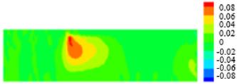
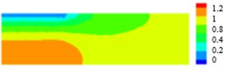
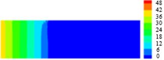
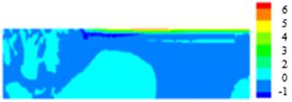
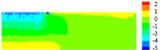
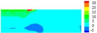
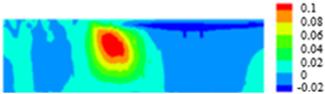
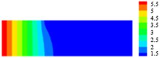
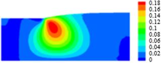
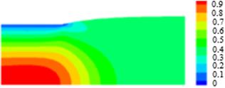
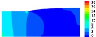
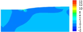
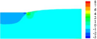
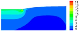
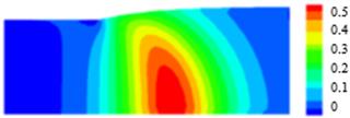
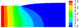
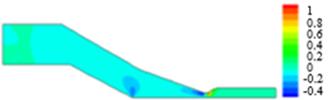
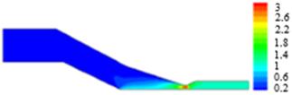
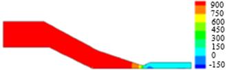
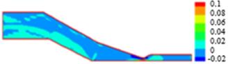
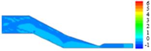
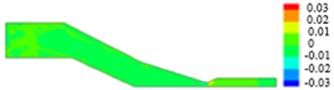
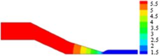
The color contour of pressure-tooling
flow with non-isothermal condition for Oldroyd-B fluid at ![]() is shown in
Figure 13. Figure 13(a) displays the radial velocity approaching zero near die
exit and the axial velocity pattern is annular shape at entrance then the flow
path develops gradually to plug model after the fluid moves to touch wire at
downstream location, so the uniform rate is the same as wire speed. When the
creep motion of polymer melt moves gently departing die, the contraction where
steep die changes to free surface causes the swell phenomenon reveal the
conservation of flow rate in accordance with Figure 13(b). Since the flow is
driven by pressure, the force is maximum at entry and reduces down to zero when
moves through the air outside the die. The measurement of pressure drop across
upstream to downstream is 960.31 as displayed in Figure 13(c). The color
contours of the maximum
is shown in
Figure 13. Figure 13(a) displays the radial velocity approaching zero near die
exit and the axial velocity pattern is annular shape at entrance then the flow
path develops gradually to plug model after the fluid moves to touch wire at
downstream location, so the uniform rate is the same as wire speed. When the
creep motion of polymer melt moves gently departing die, the contraction where
steep die changes to free surface causes the swell phenomenon reveal the
conservation of flow rate in accordance with Figure 13(b). Since the flow is
driven by pressure, the force is maximum at entry and reduces down to zero when
moves through the air outside the die. The measurement of pressure drop across
upstream to downstream is 960.31 as displayed in Figure 13(c). The color
contours of the maximum ![]() ,
, ![]() ,
, ![]() and
and ![]() referred to Figures 13(d)-13(g) are 0.84,
1.98, 6.69 and 0.03, respectively. All stresses mostly give little values
except for the neighborhood of die exit since the direction of flow is changed
instantly so all forces are transferred in the system to adjust the new
balance. The thermal is maximum at the inlet boundary and then decreased
gradually until it vanishes when the wire is coated by plastic fluid as seen in
Figure 13(h).
referred to Figures 13(d)-13(g) are 0.84,
1.98, 6.69 and 0.03, respectively. All stresses mostly give little values
except for the neighborhood of die exit since the direction of flow is changed
instantly so all forces are transferred in the system to adjust the new
balance. The thermal is maximum at the inlet boundary and then decreased
gradually until it vanishes when the wire is coated by plastic fluid as seen in
Figure 13(h).
(a) ![]()
(b) ![]()
(c) ![]()
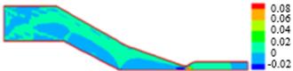
(d) ![]()
(e) ![]()
(f) ![]()
(g) ![]()
(h) ![]()
Figure 13. Annular non-isothermal pressure-tooling flow for
Oldroyd-B fluid at ![]() .
.
5. Conclusion
The simulation of wire-coating process for the pressure-tooling die, which is the representation of the extrusion procedure in industry, is studied under isothermal and non-isothermal condition. The stress equation of Oldroyd-B model is proposed with the motion of viscoelastic fluid especially for high density polyethylene, that corresponds to the selected value of material parameter. The die-swell and pressure-tooling flows are expressed via the Navier-Stokes equations in two-dimensional axisymmetric system under isothermal and non-isothermal conditions. The numerical solutions are calculated by semi-implicit Taylor-Galerkin pressure-correction finite element method with feedback of pressure-driven velocity flow. The velocity gradient recovery and the streamline-upwind/Petrov-Galerkin techniques are used to stabilized the converging solution.
For die-swell problem of non-Newtonian fluid, when Weissenberg number is increased, the viscosity and elongation are increased. The maxima of the shear stress and other stresses are located near die exit since the flows are confronted with the contraction point then the stream path is a suddenly changed to expand the radial direction known as swell phenomenon. The steep shear stress occurs at die exit because of high velocity near die exit. After the flow passes from a stick entry part to a free exit section, the singularity of severe stress and steep velocity gradients region will be appeared. The singularity point of swelling extrusion position is rough and the free surface path will become shark skin and the crack of polymer product. For pressure-tooling case, the thermal effect damages the bonding between chains of polymer so the heat affects shear rate and pressure drop. The pressure drop, shear rate and elongation of non-isothermal system are higher than those for isothermal condition as the rate of 6.73 times higher for the pressure drop, 7% higher for shear rate and 4% taller for elongation. Proper thermal regulation within the pressure-tooling process is critical to suppress premature solidification of the polymeric material and to ensure sufficient driving capability for the polymer stream to be conveyed through the die.
References
[1] V. Ngamaramvaranggul, and M. F. Webster, "Computational of free surface flows with a Taylor-Galerkin/pressure-correction algorithm," Int. J. Num. Meth. Fluids, vol. 33, pp. 936-1026, 2000. View Article
[2] N. Thongjub and V. Ngamaramvaranggul, "Simulation of die-swell flow for Oldroyd-B model with feedback semi-implicit Taylor Galerkin finite element method," KMUTNB International Journal of Applied Science Technology, vol. 8(1), pp. 55-63, 2015. View Article
[3] R. I. Tanner, "A theory of die-swell," Journal of Polymer Science Part A-2: Polymer Physics, vol. 8(12), pp. 2067-2078, 1970. View Article
[4] S. Richardson, "A stick-slip problem related to the motion of a free jet at low Reynolds numbers," Proc. Camb. Phil. Soc., vol. 67, pp. 477-489, 1970. View Article
[5] J. Thiry, F. Krier, and B. Evrard, "A review of pharmaceutical extrusion: Critical process parameters and scaling-up," International Journal of Pharmaceutics, vol. 479, pp. 227-240, 2015. View Article
[6] N. Thongjub and V. Ngamaramvaranggul, "Simulation of die-swell flow for wet powder mass extrusion in pharmaceutical process," Applied Science and Engineering Progress, vol. 13(4), pp. 354-361, 2020. View Article
[7] J. Vlachopoulos, M. Horie, and S. Lidorikis, "An evaluation of expressions predicting die swell," Trans. Soc. Rheol., vol. 16(4), pp. 669-685, 1972. View Article
[8] M. Okabe, "Fundamental theory of the semi- radial singularity mapping with applications to fracture mechanics," Comp. Meth. App. Mech. Eng., vol. 26, pp. 53-73, 1981. View Article
[9] B. Caswell and R. I. Tanner, "Wirecoating die design using finite element methods," Polym. Eng. Sci., vol. 18(5), pp. 416-421, 1978. View Article
[10] P. Wapperom and O. Hassager, "Numerical simulation of wire-coating: The influence of temperature boundary conditions," Polym. Eng. Sci., vol. 39(10), pp. 2007-2018, 1999. View Article
[11] E. Mitsoulis, "Finite element analysis of wire coating," Polym. Eng. Sci., vol. 26(2), pp. 171-186, 1986. View Article
[12] E. Mitsoulis, R. Wagner and F. L. Heng, "Numerical simulation of wire-coating low-density polyethylene: Theory and experiments," Polym. Eng. Sci., vol. 28(5), pp. 291-310, 1988. View Article
[13] I. Mutlu, P. Townsend and M. F. Webster, "Simulation of cable-coating viscoelastic flows with coupled and decoupled schemes," J. Non-Newtonian Fluid Mech., vol. 74, pp. 1-23, 1998. View Article
[14] H. Matallah, P. Townsend and M. F. Webster, "Viscoelastic computations of polymeric wire-coating flows," Int. J. Numer. Meth. Heat & Fluid Flow, vol. 12(4), pp. 404-433, 2002. View Article
[15] H. Matallah, P. Townsend and M. F. Webster, "Viscoelastic multi-mode simulations of wire-coating," J. Non-Newtonian Fluid Mech., vol. 90, pp. 217-241, 2000. View Article
[16] N. Phan-Thien, "Influence of wall slip on extrudate swell: A boundary element investigration," J. non-Newtonian Fluid Mech., vol. 26, pp. 327-340, 1988. View Article
[17] H. Baloch, H. Matallah, V. Ngamaramvaranggul and M. F. Webster, "Simulation of pressure- and tube- tooling wire-coating flows through distributed computation," Int. J. Numer. Meth. Heat & Fluid Flow, vol. 12, pp. 458-493, 2002. View Article
[18] V. Ngamaramvaranggul and S. Thenissara, "The contraction point for Phan-Thien/Tanner model of tube-tooling wire-coating flow," International journal of Physical and Mathematical Science, vol. 4(4), pp. 627-631, 2010.
[19] N. Thongjub, B. Puangkird, and V. Ngamaramvaranggul, "Simulation of slip effect with 4:1 contraction flow for Oldroyd-B fluid," Asian International Journal of Science and Technology in Production and Manufacturing Engineering, vol. 6(3), pp. 19-28, 2013.
[20] R.Y. Chang and W.L. Yang, "Numerical simulation of non-isothermal extrudate swell at high extrusion rates," J. Non-Newtonian Fluid Mech., vol. 51, pp. 1-19, 1994. View Article
[21] G. Barakos and E. Mitsoulis, "Non-isothermal viscoelastic simulations of extrusion through dies and prediction of the bending phenomenon," J. Non-Newtonian Fluid Mech., vol. 62, pp. 55-79, 1996. View Article
[22] V. Anand, "Effect of slip on heat transfer and entropy generation characteristics of simplified Phan-Thien-Tanner fluids with viscous dissipation under uniform heat flux boundary conditions: Exponential formulation," Applied Thermal Engineering, vol. 98, pp. 455-473, 2016. View Article
[23] D. Bhukta, S. R. Mishra, and M. M. Hoque, "Numerical simulation of heat transfer effect on oldroyd 8-constant fluid with wire coating analysis," Int. J. Engineering Science and Technology. vol. 19, pp. 1910-1918, 2016. View Article
[24] A. Mavi, T. Chinyoka, and A. Gill, "Modelling and analysis of viscoelastic and nanofluid effects on the heat transfer characteristics in a double-pipe counter-flow heat exchanger," Applied Sciences, vol. 12(11), 5475, pp. 1-33, 2022. View Article
[25] V. Ngamaramvaranggul and M. F. Webster, "Simulation of pressure-tooling wire-coating flows with Phan-Thien/Tanner models," Int. J. Num. Meth. Fluids., vol. 38(7), pp .677-710, 2002. View Article