Journal of Fluid Flow, Heat and Mass Transfer (JFFHMT)
ISSN: 2368-6111

Volume 12 - Year 2025 - Pages 287-304
DOI: 10.11159/jffhmt.2025.028
Simple Methods for Flow Field Computation in Perforated Tubes
Dariush Mohammadipour1, Ali Ashrafizadeh1, Hiva Hormozi1
1DOS Computational Lab, Faculty of Mechanical Engineering, K. N. Toosi University of Technology, No. 7, Pardis Street, Molasadra Ave., Tehran, Iran.
d.mohammadipour@email.kntu.ac.ir, ashrafizadeh@kntu.ac.ir, hivahormozi@email.kntu.ac.ir
Abstract - Incompressible flow in perforated tubes has many industrial applications including jet engine cooling. Numerical solution methods for multi-dimensional flow models are often prohibitively expensive. Therefore, engineers are interested in simple and rapid computational methods that are applicable in determining velocity and pressure fields in perforated tubes. To respond to this demand, the present paper introduces a number of such methods. Furthermore, using the aforementioned simple methods, the effects of the distribution and diameters of circular holes in a perforated tube with a closed end on the flow field are thoroughly investigated. It is shown that using a one-dimensional ideal flow model, analytical solution is possible when the holes have equal diameters and are uniformly distributed (Case 1). A semi-analytical procedure is presented for the ideal flow model when the holes are non-uniformly distributed and/or have various diameters (Case 2). To take the effects of fluid viscosity into consideration, viscous flow in a perforated tube is solved using a numerical solution approach (Case 3). A criterion is provided regarding the applicability of the ideal flow model. Comparison with experimentally-obtained pressure field in a perforated tube shows that the maximum error of ideal flow model, when applicable, is less than 20%. The numerical viscous flow solution is also validated and excellent match with the reference data is observed.
Keywords: Manifolds, Perforated tubes, Ideal flow.
© Copyright 2025 Authors - This is an Open Access article published under the Creative Commons Attribution License terms Creative Commons Attribution License terms. Unrestricted use, distribution, and reproduction in any medium are permitted, provided the original work is properly cited.
Date Received: 2025-06-08
Date Revised: 2025-07-01
Date Accepted: 2025-07-16
Date Published: 2025-08-11
Nomenclature
|
tube cross section (m2) |
|
|
Aj |
hole cross section (m2) |
|
|
unknown coefficients in Eq. (24) |
|
CV |
Control Volume |
|
|
Constant coefficient in Eq. (2) |
|
d |
hole diameter (m) |
|
D |
tube diameter (m) |
|
Eu |
Euler number |
|
|
x-dependent functions in Eq. (1) |
|
|
Friction factor |
|
|
dimensionless friction factor |
|
|
ratio of manifold length to CV length (L/s) |
|
|
ratio of manifold to hole diameter (D/d) |
|
|
the ratio of cross-sectional area of the tube to the total discharge area |
|
i, j |
counter |
|
k |
Pressure recovery factor |
|
L |
length of the tube (m) |
|
n |
number of holes |
|
|
pressure (pa) |
|
|
atmospheric pressure (pa) |
|
Pj |
dimensionless pressure defined in Eq. (23) |
|
P0 |
dimensionless manifold inlet pressure |
|
|
Inlet Reynolds number |
|
|
Length of a control volume (m) |
|
t |
manifold thickness (m) |
|
u |
velocity in manifold (m/s) |
|
|
dimensionless velocity in manifold (u/u0) |
|
|
inlet flow velocity (m/s) |
|
|
jet velocity(m/s) |
|
|
average jet velocity (m/s) |
|
|
dimensionless jet velocity |
|
x |
axial coordinate (m) |
|
X |
dimensionless axial coordinate |
Greek symbols
|
ρ |
density (kg/m3) |
|
λ |
Parameter defined in Eq. (7) |
|
|
dimensionless parameter defined in Eq. (12) |
1. Introduction
Manifolds are widely used to distribute fluid in flow systems. Perforated tubes, shown in Figure1, constitute a subgroup of the manifolds with many industrial applications. For example, they are used in gasification and drip irrigation systems [1], [2], injection of fluids into the core of a nuclear reactor for emergency shutdown [3], [4], injection of bubbles to create a homogeneous multiphase reaction in chemical reactors [5], [6], reducing the exhaust noise in internal combustion engines [7], [8], and cooling via jet impingement. A particularly interesting application of the impinging jets is in the active clearance control system of aircraft engines [9], [10]. Figure 2 shows the perforated tubes (impingement pipes) that are used to cool down the casing of a jet engine turbine. Manifolds are used to carry the cooling air from a front section of the engine and distribute it around the casing via perforated tubes. A number of small holes near the closed end of a perforated tube are shown in Figure 3. Figure 1 (a), is a model of the actual pipe shown in Figure 3. The sizes of the holes and the way they are distributed along the tube, strongly affect the impinging jet velocities and hence the cooling effectiveness and uniformity.
(a)
(b)
Figure 1. A simple perforated tube with a closed-end, a) 3D view, b) 2D view.
Figure 2 Perforated tubes (impingement pipes) used to cool down the low-pressure gas turbine casing in a jet engine [10].
Figure 3. Part of a closed end perforate tube used in an impingement cooling system.
The flow field details in a perforated tube can be obtained using computational fluid dynamics [11]-[17] . These solutions provide detailed information about the flow field; However, the computational cost can be very high, especially for tubes with a large number of holes [18-19]. Therefore, more versatile tools and methods are preferred for rapid engineering estimations.
Discrete and continuous mathematical models have also been developed for flow analysis in perforated tubes [20]-[30]. The flow governing equations in these relatively simple one-dimensional models are obtained by enforcing fluid mass and momentum conservations for the control volumes defined around the holes, as shown in Figure 4.
(a)
(b)
Figure 4. Control volumes around the holes in a perforated tube, a) uniformly distributed holes, b) non-uniformly distributed holes.
Wang [21] has shown that a rather general one-dimensional flow model for incompressible flow in perforated tubes is obtained in which fluid viscosity, discharge coefficients for the holes, and the pressure recovery effect due to discharged flow from the holes, are all taken into consideration. The mathematical structure of the equation for the axial flow velocity along the perforated tube in such a one-dimensional model is as follows:
In this equation, ![]() to
to ![]() are
are ![]() -dependent
functions, and
-dependent
functions, and ![]() is the axial fluid velocity as a
function of
is the axial fluid velocity as a
function of ![]() (the
coordinate along the tube’s axis). To derive Eq. (1), it is assumed that the
holes are very close to each other so that second and higher-order powers of
the control volume lengths are negligible.
(the
coordinate along the tube’s axis). To derive Eq. (1), it is assumed that the
holes are very close to each other so that second and higher-order powers of
the control volume lengths are negligible.
Equation (1) is a highly non-linear second-order differential equation with variable coefficients and is difficult to solve analytically. For the uniformly distributed equal-size holes along the tube, a rather simpler equation, Eq. (2), is obtained.
In Eq. (2) ![]() and
and ![]() are variable coefficients, proportional
to the pressure recovery and the local friction factor, respectively. Even this
simpler mathematical model is again a non-linear second order differential
equation with variable coefficients and is still difficult to solve
analytically.
are variable coefficients, proportional
to the pressure recovery and the local friction factor, respectively. Even this
simpler mathematical model is again a non-linear second order differential
equation with variable coefficients and is still difficult to solve
analytically.
Wang et al. [21] have provided useful information regarding the possible solution procedures for the fluid velocity along the tube for a subset of Eq. (2). Some information regarding the physics of the flow, as predicted by one-dimensional models and some valuable results regarding the pressure and velocity fields are provided in [21], [23], [31] .
Here, we first drastically simplify the general one-dimensional flow model in an attempt to separately investigate the effects of the physical properties and geometrical parameters on the flow distribution in a perforated tube. The ideal flow model allows us to focus on the geometrical effects. Viscosity-related terms can then be included in the model to investigate the physical properties and effects. This approach helps to think more fundamentally about the applicability of the models and possible solution strategies and hopefully enrich the already rich research resources on the solution of this problem.
The flow of the information in this paper is as follows: in the next section, Section 2, a one dimensional mathematical model is derived for the ideal flow in a segment of a perforated tube.
Section 3 provides an analytical
solution for the axial flow velocity of an ideal fluid along a tube with
uniformly distributed holes with equal diameters. In Section 4, a
semi-analytical computational method is presented to solve the equation for ![]() in a perforated tube with
non-uniformly distributed holes carrying ideal fluid. Afterwards, in Section 5
a numerical solution method is presented to solve the equation for
in a perforated tube with
non-uniformly distributed holes carrying ideal fluid. Afterwards, in Section 5
a numerical solution method is presented to solve the equation for ![]() in a perforated tube carrying a
viscous fluid. Section 6, is devoted to the presentation of computational
results in all cases. Finally, Section 7 wraps up the paper with some
concluding remarks.
in a perforated tube carrying a
viscous fluid. Section 6, is devoted to the presentation of computational
results in all cases. Finally, Section 7 wraps up the paper with some
concluding remarks.
2. An Ideal Flow Mathematical Model
By ignoring the viscous effects on the flow field and assuming a perfect discharge scenario, i.e., normal and loss-free discharge of the fluid from the holes, the following governing equations are obtained for the flow in a small segment of the pipe, defined as a control volume around a typical hole, as shown in Figure 5 [21].
Figure 5. Inviscid flow momentum balance for a typical control volume defined in a perforated tube.
For the sake of further simplicity,
the density is assumed to be one ![]() and in this Section the circular
holes are similar and uniformly distributed.
and in this Section the circular
holes are similar and uniformly distributed.
Mass conservation:
![]() (3)
(3)
Momentum conservation:
Bernoulli for the discharged flow:
![]() (5)
(5)
In these equations, ![]() is the fluid velocity along the tube,
is the fluid velocity along the tube, ![]() is
the discharged jet velocity,
is
the discharged jet velocity, ![]() is
the fluid pressure along the tube,
is
the fluid pressure along the tube, ![]() is the ambient pressure,
is the ambient pressure, ![]() is the length of the control volume,
equal to the distance between two neighbor holes in this case, and
is the length of the control volume,
equal to the distance between two neighbor holes in this case, and ![]() and
and ![]() are
the tube and hole diameters, respectively. Using Eqs. (3) to (5), the following
differential equation is obtained for the axial flow velocity in the tube:
are
the tube and hole diameters, respectively. Using Eqs. (3) to (5), the following
differential equation is obtained for the axial flow velocity in the tube:
![]() (6)
(6)
In which:
![]() (7)
(7)
Using ![]() (the fluid inlet velocity) and
(the fluid inlet velocity) and ![]() (the
tube length) as characteristic velocity and length scales, the non-dimensional
form of Eq. (6) is obtained as follows:
(the
tube length) as characteristic velocity and length scales, the non-dimensional
form of Eq. (6) is obtained as follows:
![]() (8)
(8)
In which
![]() (9)
(9)
![]() (10)
(10)
![]() (11)
(11)
Note that:
![]() (12)
(12)
In which:
![]() (13)
(13)
![]() (14)
(14)
It is now evident that the ideal flow
distribution in a perforated tube with fixed length ![]() and
fixed diameter
and
fixed diameter ![]() is governed by two non-dimensional
geometrical parameters, i.e.
is governed by two non-dimensional
geometrical parameters, i.e. ![]() . In this study,
. In this study, ![]() and
and ![]() are assumed constants in all test
cases unless otherwise stated. Note that
are assumed constants in all test
cases unless otherwise stated. Note that ![]() corresponds to the number of holes in
this case. Therefore, for ideal flow in a perforated tube with uniformly
distributed equal-size circular holes, the number and diameter of holes govern
the fluid velocity distribution through Eq. (8).
corresponds to the number of holes in
this case. Therefore, for ideal flow in a perforated tube with uniformly
distributed equal-size circular holes, the number and diameter of holes govern
the fluid velocity distribution through Eq. (8).
Equation (8) is a second-order differential equation and needs two boundary conditions. Assuming a perforated tube with a closed end, the non-dimensional boundary conditions are as follows:
![]() (15)
(15)
![]() (16)
(16)
The solution of Eq. (8) with the
boundary conditions (15 and 16) is discussed in Section 3. Note that by
determining the ![]() function, the jet velocities can be
calculated via Eq. (3), and the pressure field is then obtained using Eq. (5).
Looking at the equations and thinking about the physics of the flow in this
simple model, it is pretty clear that the flow distribution is the result of
interactions between the flow inertia (through fluid velocity along the tube)
and pressure forces. The closed end of the tube has a particularly important
role in the pressure recovery, given that all of the kinetic energy at
function, the jet velocities can be
calculated via Eq. (3), and the pressure field is then obtained using Eq. (5).
Looking at the equations and thinking about the physics of the flow in this
simple model, it is pretty clear that the flow distribution is the result of
interactions between the flow inertia (through fluid velocity along the tube)
and pressure forces. The closed end of the tube has a particularly important
role in the pressure recovery, given that all of the kinetic energy at ![]() is converted to internal (pressure)
energy. In fact, the geometrical features of the tube and holes constrain the
pressure field so that the fluid inertia is restrained appropriately and the
mass conservation is satisfied. This is, in fact, an explanation for the role
of the pressure in incompressible flow.
is converted to internal (pressure)
energy. In fact, the geometrical features of the tube and holes constrain the
pressure field so that the fluid inertia is restrained appropriately and the
mass conservation is satisfied. This is, in fact, an explanation for the role
of the pressure in incompressible flow.
To better understand the importance of the role of the pressure and the flow adjustment due to the sizes and numbers of the holes, let's naively assume that we just need to take care of the mass conservation in this simple problem. For equal-size circular holes in a tube similar to the one shown in Figure 1, the average discharged-jet velocity is easily calculated as follows:
![]() (17)
(17)
Note that ![]() is defined as the ratio of the
cross-sectional area of the tube (
is defined as the ratio of the
cross-sectional area of the tube (![]() to the total discharge area, i. e. the
sum of the holes’ areas (
to the total discharge area, i. e. the
sum of the holes’ areas (![]() . It is obvious that the
. It is obvious that the ![]() parameter, as defined in Eq. (17), is
an important characteristic parameter for perforated tubes. For example, if the
average jet velocity (
parameter, as defined in Eq. (17), is
an important characteristic parameter for perforated tubes. For example, if the
average jet velocity (![]() )
needs to be significantly higher than the tube’s inlet velocity (
)
needs to be significantly higher than the tube’s inlet velocity (![]()
![]() has to be significantly higher than
one. Therefore, this parameter defines a continuity-based average jet velocity
for perforated tubes with equal-size circular holes. We will compare the
calculated jet velocities in a perforated tube with equal-size circular holes
with
has to be significantly higher than
one. Therefore, this parameter defines a continuity-based average jet velocity
for perforated tubes with equal-size circular holes. We will compare the
calculated jet velocities in a perforated tube with equal-size circular holes
with ![]() ,
i.e the continuity-based average velocity, to see how the pressure field
affects the flow distribution through the momentum balance.
,
i.e the continuity-based average velocity, to see how the pressure field
affects the flow distribution through the momentum balance.
With this background information
regarding the perforated tubes with uniformly distributed holes, it can be
shown that for variable pitch (distance between the holes) and hole diameter ![]() Eq. (8) is no longer valid throughout
the tube, and the following equation needs to be solved for the ideal
(inviscid) flow assumption described previously:
Eq. (8) is no longer valid throughout
the tube, and the following equation needs to be solved for the ideal
(inviscid) flow assumption described previously:
![]() (18)
(18)
The coefficients of the second and the
third terms of Eq. (18) are not constant values, and more complicated
analytical methods are needed to solve this equation. The analytical solution,
if obtained, might not be in a simple mathematical form. For example, the
solution might be in the form of a power series. This further mathematical
complexity is because the holes play a much more complicated role in the flow
distribution along the perforated tube in this case. The good news is that we
do not need to solve Eq. (18) analytically. In Section 4, it is shown that Eq.
(8) is still applicable locally. We can take the variations of ![]() and
and
![]() into
account by advising a semi-analytical approach in which consistency conditions
are satisfied at the boundary faces of control volumes that enclose the holes.
into
account by advising a semi-analytical approach in which consistency conditions
are satisfied at the boundary faces of control volumes that enclose the holes.
Now, let’s keep S and d constants (uniform spacing and equal-size holes) and include the fluid viscosity effect to obtain a third simplified mathematical model. For a perforated tube with uniformly distributed equal-size holes, carrying a viscous fluid, the following one-dimensional flow model is obtained:
In Eq. (19), ![]() represents
represents
![]() , in which
, in which ![]() is
the friction factor. While pressure drop due the viscosity is considered in
this model, other real flow effects such as pressure recovery factors and
discharge coefficients for the holes are not taken into consideration.
is
the friction factor. While pressure drop due the viscosity is considered in
this model, other real flow effects such as pressure recovery factors and
discharge coefficients for the holes are not taken into consideration.
Hereafter, for the sake of brevity, the tube with uniformly distributed equal-size holes carrying inviscid fluid is called Case 1, the tube with non-uniformly distributed and/or variable-size holes carrying inviscid fluid is called Case 2, and the tube with uniformly distributed equal-size holes carrying viscous fluid is called Case 3.
3. Analytical Solution of the Equation for Fluid Velocity in Case 1
Equation (8) with boundary conditions (15) and (16) can be solved analytically. The standard method for finding the general solution of Eq. (8) is by assuming the solution structure and then solving the characteristic equation. During this process, two integration constants appear in the general solution. These constants are obtained by constraining the general solution to satisfy the boundary conditions (15) and (16). A solution that satisfies all of the constraints, i.e., Eq. (8) and boundary conditions (15) and (16), is as follows:
![]() (20)
(20)
Using Eq. (20) and the non-dimensional form of Eq. (3), non-dimensional jet velocities are obtained as given below:
![]() (21)
(21)
Discrete coordinate value described by ![]() in Eq. (21), represents the axial
coordinate of the
in Eq. (21), represents the axial
coordinate of the ![]() hole and
hole and ![]() is the jet velocity at that position.
is the jet velocity at that position.
Using Eq. (21) and the non-dimensional form of Eq. (5),
non-dimensional pressure at the ![]() position is obtained as follows:
position is obtained as follows:
![]() (22)
(22)
The non-dimensional relative pressure in Eq. (22) is defined as given below:
![]() (23)
(23)
Equations (20), (21), and (22) can be easily plotted for various ![]() values.
Given the relation between
values.
Given the relation between ![]() ,
, ![]() and
and ![]() , we can also separately change
, we can also separately change ![]() and
and ![]() to investigate the effects of the
number of holes and hole diameter on the velocity and pressure fields in this
case. Note that both
to investigate the effects of the
number of holes and hole diameter on the velocity and pressure fields in this
case. Note that both ![]() and
and
![]() are assumed constants in the current
study.
are assumed constants in the current
study.
The simplified model in Case 1 leads to a governing equation that depends only on geometric parameters. This not only allows for a separate analysis of how geometrical features, such as hole spacing and diameter, affect the flow distribution without interference from physical properties like viscosity, but also provides an analytical solution that serves as a reliable initial estimate for more complex, viscosity-dependent cases.
4. Semi-Analytical Solution of the Equation for Fluid Velocity in Case 2
Instead of seeking an analytical solution to Eq. (18), which is
valid throughout a perforated tube with variable ![]() ,
we can still assume that Eq. (8) is locally valid in a discrete solution
domain. Therefore, the general analytical solution of Eq. (8) in the
,
we can still assume that Eq. (8) is locally valid in a discrete solution
domain. Therefore, the general analytical solution of Eq. (8) in the ![]() control volume provides the velocity
distribution throughout that control volume. In contrast to Case 1, the
control volume provides the velocity
distribution throughout that control volume. In contrast to Case 1, the ![]() parameter
is not a constant value in this case, and piecewise analytical solutions have to be sought in Case 2.
parameter
is not a constant value in this case, and piecewise analytical solutions have to be sought in Case 2.
The general solution of Eq. (8) for the velocity distribution in
the ![]() control volume can be written in the
following form:
control volume can be written in the
following form:
![]() (24)
(24)
Equation (24) needs two boundary conditions to provide the
velocity distribution in the ![]() control volume. To explain how the
constants in Eq. (24) are determined, let’s consider a very simple perforated
tube shown in Figure 6. The velocity distribution throughout this tube is
described by the following velocity distribution segments associated with
control volumes 1, 2, and 3 respectively:
control volume. To explain how the
constants in Eq. (24) are determined, let’s consider a very simple perforated
tube shown in Figure 6. The velocity distribution throughout this tube is
described by the following velocity distribution segments associated with
control volumes 1, 2, and 3 respectively:
![]() (25)
(25)
![]() (26)
(26)
![]() (27)
(27)
Note that there are six unknowns, i.e. ![]() and
and ![]() for
for ![]() , that need to be determined.
, that need to be determined.
Figure 6. A control volume-based discrete model using piecewise analytical solutions for the fluid velocity in a perforated tube.
In this case the closure equations, required to close the system,
are obtained from the boundary conditions and continuity constraints for the
velocity and velocity slope (rate of change of velocity with respect to ![]() ) at the control surfaces. These
constraints for the simple case shown in Figure 6 are given below:
) at the control surfaces. These
constraints for the simple case shown in Figure 6 are given below:
The inlet boundary condition ( ![]() ):
):
![]() (28)
(28)
The continuity constraint on
the velocity magnitude at ![]() :
:
![]() (29)
(29)
The continuity constraint on
the velocity slope at ![]() :
:
![]() (30)
(30)
The continuity constraint on
the velocity magnitude at ![]() :
:
![]() (31)
(31)
The continuity constraint on
the velocity slope at ![]() :
:
![]() (32)
(32)
The boundary condition at the
end of the tube (![]() )
)
![]() (33)
(33)
Equations (28) to (33) provide six constraints for the six unknown coefficients in Eqs. (25) to (27). Using the general solution structure given in Eq. (24), the aforementioned constraints can be written in expanded forms. For example, the expanded form of Eq. (30) is as follows:
![]() (34)
(34)
In general, for ![]() control
volumes, there are
control
volumes, there are ![]() unknown constants associated with the
segmental velocity distributions. These unknowns are obtained by simultaneous
solution of a set of linear algebraic equations. The elements of the
coefficient matrix in the set of equations depend solely on the
unknown constants associated with the
segmental velocity distributions. These unknowns are obtained by simultaneous
solution of a set of linear algebraic equations. The elements of the
coefficient matrix in the set of equations depend solely on the ![]() and
and ![]() values. The boundary conditions
appear in the right-hand side vector of the matrix equation corresponding to
the set of linear algebraic equations for the unknown
values. The boundary conditions
appear in the right-hand side vector of the matrix equation corresponding to
the set of linear algebraic equations for the unknown ![]() values.
values.
Equation (35) shows the general structure of the linear system in
the matrix form for the simple case shown in Figure 6. Non-zero values in the
coefficient matrix are represented by the multiplication sign ![]() .
.
 (35)
(35)
The solver options in MATLAB can easily solve the equation set. Row interchange before the solution might be necessary to avoid singularities. The solver takes care of such matrix structural problems before the solution.
This semi-analytical formulation enables efficient evaluation of the velocity field in perforated tubes with non-uniform perforation properties, without relying on full 3D CFD simulations. While typical CFD studies require millions of mesh elements even for relatively short manifolds (e.g., 20 million cells for 20 holes [14]), the present approach reduces the problem to a tractable set of linear algebraic equations with significantly lower computational cost. This makes it a practical and scalable alternative for preliminary design and parametric studies.
5. Numerical Solution of the Equation for Fluid Velocity in Case 3
In this case, Eq. (19) is the mathematical model for the flow in a
perforated tube with uniformly distributed equal-size holes. Note that while ![]() is constant, the parameter F changes along the tube due to the variation of
friction factor
is constant, the parameter F changes along the tube due to the variation of
friction factor ![]() .
To employ Eq. (19) and calculate the velocity distribution along the tube, we
try to solve this equation within the individual control volumes. Assuming a
configuration similar to the one shown in Figure 6, the velocity field within
the
.
To employ Eq. (19) and calculate the velocity distribution along the tube, we
try to solve this equation within the individual control volumes. Assuming a
configuration similar to the one shown in Figure 6, the velocity field within
the ![]() control volume is governed by the
following constraints:
control volume is governed by the
following constraints:
![]() (36)
(36)
![]() (37)
(37)
![]() (38)
(38)
Note that in this case we do not have analytical solution for the
governing equation. This has two implications. First, we need to solve Eq. (36)
using numerical methods. And, second, an iterative approach is required to
impose the continuity constraints on the facial values of velocity and velocity
slope. For the numerical solution of Eq. (36), the shooting method, assisted
with the well-known 4th-order Runge-Kutta method, is employed. This is carried
out by defining a number of auxiliary points within control volumes. These
points are uniformly distributed and the distance between two consecutive
points is shown by ![]() .
.
Again, let’s consider the flow in the very simple perforated tube shown in Figure 6. The iterative numerical solution approach starts with providing guessed velocity values at all internal faces (control surfaces) as follows:
![]() (39)
(39)
![]() (40)
(40)
With the guessed velocity values at control surfaces, i.e. ![]() and
and ![]() , Eq. (36) can be solved in all three
control volumes in Figure 6, to obtain
, Eq. (36) can be solved in all three
control volumes in Figure 6, to obtain ![]() and
and ![]() , i.e. the velocity distributions
inside control volumes. Here, the subscript in
, i.e. the velocity distributions
inside control volumes. Here, the subscript in ![]() ,
, ![]() , represents the control volume number
and the superscript represents the iteration number. For example,
, represents the control volume number
and the superscript represents the iteration number. For example, ![]() represents the velocity distribution
in the first control volume at the first iteration.
represents the velocity distribution
in the first control volume at the first iteration.
Given the fact that guessed velocity values have been used at the
control surfaces, a correction procedure is required to update the boundary
values used to solve Eq. (36) in the control volumes. This is done by requiring
the continuity of the velocity slopes at internal control surfaces as given in
Eqs. (30) and (32). For example, the following constraint should be imposed at ![]() in Figure 6:
in Figure 6:
![]() (41)
(41)
To carry out this task, the numerical solutions at the neighboring control volumes are employed as follows:
![]() (42)
(42)
![]() (43)
(43)
Note that there is no guarantee that Eq. (41) is satisfied when
the velocity slopes are calculated using Eqs. (42) and (43). The difference
between the current estimation of ![]() and
and ![]() can now be used to update the fluid
velocity at
can now be used to update the fluid
velocity at ![]() :
:
 (44)
(44)
To better understand the rationale behind Eq. (44), one might
think of it as an interpolation formula that takes the average of two truncated
Taylor series approximations of ![]() , using the most recent available
solutions in neighboring control volumes. Similar procedure is carried out at
all other internal control surfaces. The iterative process ends when the
velocity slope continuity is satisfied at all internal control surfaces. The
actual convergence criterion that is implemented in this study is as follows:
, using the most recent available
solutions in neighboring control volumes. Similar procedure is carried out at
all other internal control surfaces. The iterative process ends when the
velocity slope continuity is satisfied at all internal control surfaces. The
actual convergence criterion that is implemented in this study is as follows:
![]() (45)
(45)
Equation (45) means that upon convergence, the difference between
the right and left estimates for the velocity slope values at control surfaces
are all less than ![]() The number of auxiliary points that
are used for the numerical integration of Eq. (36) in control volumes is user
defined. In this study, 99 auxiliary points are used within each control
volume.
The number of auxiliary points that
are used for the numerical integration of Eq. (36) in control volumes is user
defined. In this study, 99 auxiliary points are used within each control
volume.
Additionally, to calculate the friction factor (𝑓), the well-known Darcy friction factor correlations can be used.
![]() (46)
(46)
![]() (47)
(47)
![]() (48)
(48)
Figure (7) shows the flow chart of the iterative numerical solution in the simple test case shown in Figure 6.
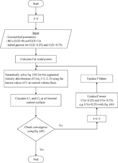
Figure 7. Flow chart of the iterative numerical solution algorithm in Case 3 for the perforated tube model shown in Figure 6.
4. Results and Discussions
6.1. Analytical Solution for the Case 1
Equation (20), which is the analytical solution of Eq. (8), is used to draw the non-dimensional fluid velocity distribution along the tube for three different values of ![]() as
shown in Figure 8. As expected,
as
shown in Figure 8. As expected, ![]() tends to be closer to a linear
distribution for smaller
tends to be closer to a linear
distribution for smaller ![]() values.
In fact, for the limiting case of
values.
In fact, for the limiting case of ![]() , the velocity distribution is
strictly linear. For higher values of
, the velocity distribution is
strictly linear. For higher values of ![]() ,
the velocity distribution is not linear, pointing to a non-uniform discharge
from the holes. It should be noted that symbols used in Figure 8 are used to
show the fluid velocities at a few
,
the velocity distribution is not linear, pointing to a non-uniform discharge
from the holes. It should be noted that symbols used in Figure 8 are used to
show the fluid velocities at a few ![]() locations along the tube.
locations along the tube.
Figure 8. Ideal flow distribution in a perforated tube with uniformly distributed equal-size holes (Case 1).
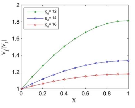
Figure 9 shows the distribution of the discharge velocities from
the holes. Equation (21) is used to draw the diagrams, and jet velocities are
scaled using the first jet velocity for better comparison. Note that for ![]() the jet velocities are nearly equal.
In contrast, jet velocities near the end of the tube are considerably greater
than the velocity of the first jet for
the jet velocities are nearly equal.
In contrast, jet velocities near the end of the tube are considerably greater
than the velocity of the first jet for ![]()
Figure 9. Non-dimensional jet velocities in Case 1, normalized with the velocity of the first jet.
The normalized relative pressure distribution along the tube can also be drawn using Eq. (22), as shown in Figure 10. The build-up of pressure at the closed end of the tube is observed in all cases.
Figure 10. Non-dimensional relative pressure distribution along the tube in Case 1.
As mentioned before and given in Eq. (12), the parameter ![]() is
a function of two geometrical parameters represented by
is
a function of two geometrical parameters represented by ![]() and
and ![]() . For a perforated tube with a fixed
length and diameter,
. For a perforated tube with a fixed
length and diameter, ![]() varies with S and
varies with S and ![]() varies with d. It makes sense to see
how these non-dimensional parameters affect the flow distribution in case 1.
varies with d. It makes sense to see
how these non-dimensional parameters affect the flow distribution in case 1.
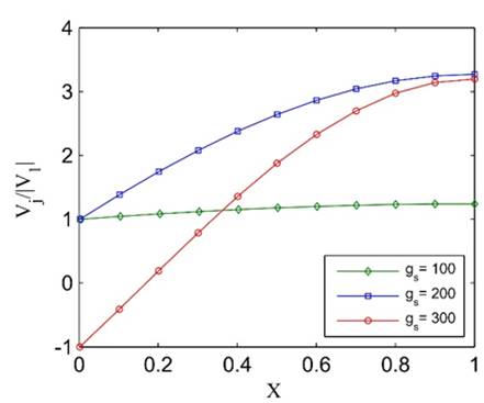
In Figure 11 (a), the diameters of a fixed number of holes
(corresponding to ![]() ) are changed to see the effect of
) are changed to see the effect of ![]() (or
(or ![]() )
on the axial flow velocity. In a similar manner, the number of equal size holes
(corresponding to
)
on the axial flow velocity. In a similar manner, the number of equal size holes
(corresponding to ![]() ) are changed in Figure 11 (b) to see
the effect of
) are changed in Figure 11 (b) to see
the effect of ![]() (or
(or ![]() )
on the axial flow velocity. Obviously, the corresponding values of
)
on the axial flow velocity. Obviously, the corresponding values of ![]() can
be easily calculated using Eq. (12) in each case. An important observation in Figure
11 (b) is for the case
can
be easily calculated using Eq. (12) in each case. An important observation in Figure
11 (b) is for the case ![]() and
and ![]() , which corresponds to
, which corresponds to ![]() . Note that for this case, the axial
velocity increases in the initial section of the tube. This is possible only if
the flow is sucked into the holes instead of being discharged. In fact, the
initial part of the perforated tube with
. Note that for this case, the axial
velocity increases in the initial section of the tube. This is possible only if
the flow is sucked into the holes instead of being discharged. In fact, the
initial part of the perforated tube with ![]() acts like a jet pump instead of
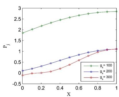
discharging the fluid. Corresponding values of normal velocities across the
holes and pressure distributions are shown in Figs. 12 and 13, respectively. In
some cases, negative values of velocity and pressure are consistent with the
observations in Figure 11.
acts like a jet pump instead of
discharging the fluid. Corresponding values of normal velocities across the
holes and pressure distributions are shown in Figs. 12 and 13, respectively. In
some cases, negative values of velocity and pressure are consistent with the
observations in Figure 11.
(a)
(b)
Figure 11. Axial flow velocity
distribution in Case 1, (a) ![]() , (b)
, (b) ![]()
(a)
(b)
Figure 12. Jet velocity distribution in Case 1, (a) ![]() , (b)
, (b) ![]()
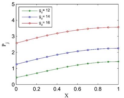
(a)
(b)
Figure 13. Pressure distribution in Case 1, (a) ![]() , (b)
, (b) ![]()
6.1.1. Understanding the Role of the Pressure Field
As mentioned before, the pressure field affects the flow field so
that the jet velocities are not the same as the continuity-based average
discharge velocity ![]() .
In Figure 14, jet velocities obtained for
.
In Figure 14, jet velocities obtained for ![]() and
and ![]() , are compared to
, are compared to ![]() .
Note that due to the pressure build-up near the end of the tube, velocities of
the jets coming out of the holes after
.
Note that due to the pressure build-up near the end of the tube, velocities of
the jets coming out of the holes after ![]() are higher than the average velocity
are higher than the average velocity ![]() .
Necessarily, due to the mass conservation constraint, the jet velocities near
the tube’s inlet are less than
.
Necessarily, due to the mass conservation constraint, the jet velocities near
the tube’s inlet are less than ![]() .
This is how the pressure field competes with the inertia in this simple flow
model to re-distribute the fluid between the holes.
.
This is how the pressure field competes with the inertia in this simple flow
model to re-distribute the fluid between the holes.
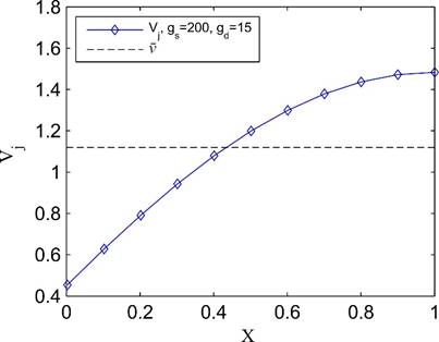
Figure 14. Effect of the pressure field on the flow distribution between holes in Case 1.
6.2. Validation of the Semi-Analytical Solution Approach
To validate the semi-analytical solution approach, described in Section 4, this method is used to solve the flow problem in Case 1. Comparison between the analytical solution (A) and semi-analytic solution (SA) in Figure 15 shows that solutions from the two methods match perfectly. Once again, it should be remembered that U values at just a few locations along the tube are marked with symbols for clarity.
Figure 15. Validation of the semi-analytical method.
6.3. Semi-Analytical Solutions for the Case 2
6.3.1. Effect
of Non-Uniformity in Hole’s Spacing (![]() )
)
The semi-analytic solution method makes it possible to use the
analytical solutions in the control volumes in a piecewise/discrete manner.
Therefore, the sizes of the control volumes, or equivalently distances between
the holes, need not be equal. Two extreme scenarios regarding the non-uniform
distribution of equal-size holes (![]() ) are shown in Figure 16. In the upper
tube in Figure 16, the holes are getting closer toward the end of the tube in a
linear manner (so that
) are shown in Figure 16. In the upper
tube in Figure 16, the holes are getting closer toward the end of the tube in a
linear manner (so that ![]() ), and, in the lower tube, the
distances between the holes increase linearly (so that
), and, in the lower tube, the
distances between the holes increase linearly (so that ![]() ). Note that
). Note that ![]() is
the number of holes. We call these two scenarios as contracting and expanding
scenarios, respectively.
is
the number of holes. We call these two scenarios as contracting and expanding
scenarios, respectively.
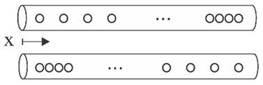
Figure 16. Two scenarios for non-uniform distribution of
equal-size holes (![]() ).
).
Figure 17 (a) shows the effect of the variable spacing on the jet
velocity distribution, and Figure 17 (b) shows the associated pressure
distributions along the tube. Note that for the expanding scenario (![]() ), which corresponds to ascending
), which corresponds to ascending ![]() values, higher jet velocities are
obtained near the end of the tube and for the contracting scenario (
values, higher jet velocities are
obtained near the end of the tube and for the contracting scenario (![]() ), which corresponds to descending
), which corresponds to descending ![]() values, smaller jet velocities are
obtained closer to the end of the tube as expected. This means that changing
the spacing between equal-size holes can affect or control the pressure
distribution and jet velocities along the tube.
values, smaller jet velocities are
obtained closer to the end of the tube as expected. This means that changing
the spacing between equal-size holes can affect or control the pressure
distribution and jet velocities along the tube.
(a)
(b)
Figure 17. Distribution of jet velocities (a) and pressure
distribution (b) for non-uniform distribution of holes (![]() ).
).
6.3.2. Effect
of the Non-Uniformity in Holes’ Sizes (![]() )
)
To examine the effects of the hole size distribution on the flow
field in a perforated tube, again, two scenarios are considered, as shown in Figure
18. Two extreme scenarios regarding the variable-size holes that are uniformly
distributed along the tube (![]() ), are shown in Figure 18. In the
upper tube in Figure 18, the holes are getting smaller towards the end of the
tube in a linear manner (so that
), are shown in Figure 18. In the
upper tube in Figure 18, the holes are getting smaller towards the end of the
tube in a linear manner (so that ![]() ), and in the lower tube, the holes’
diameters increase linearly (so that
), and in the lower tube, the holes’
diameters increase linearly (so that ![]() ).
).
Figure 18. Two scenarios for the variation of holes’ diameters
along the tube (![]() ).
).
Figure 19 (a) shows the effect of the diameter variation of the holes on the jet velocity distribution, and Figure 19 (b) shows the associated pressure distributions along the tube. Again, it is noted that the hole diameter variation can be used to control the flow distribution in a perforated tube.
(a)
(b)
Figure 19. Distribution of jet velocities (a) and pressure
distribution (b) for unequal-size holes evenly distributed along the tube (![]() ).
).
Note that the distribution functions used to determine the ![]() and
and ![]() values, i.e.
values, i.e. ![]() and
and ![]() functions, need not be linear in Case
(2), and non-linear distributions provide more flexibility to control the
pressure and flow distribution along the perforated tube.
functions, need not be linear in Case
(2), and non-linear distributions provide more flexibility to control the
pressure and flow distribution along the perforated tube.
6.3.3. The
Cumulative Effect of ![]() and
and ![]()
Based on the results presented in the previous Sections, i.e.,
Sections 6.3.1 and 6.3.2, it is also possible to select proper values of ![]() and
and ![]() so that a rather uniform pressure
distribution, and hence uniform jet velocities along the tube, is obtained.
Figure 20 shows one possible scenario: an ascending
so that a rather uniform pressure
distribution, and hence uniform jet velocities along the tube, is obtained.
Figure 20 shows one possible scenario: an ascending ![]() function combined with a descending
function combined with a descending ![]() . The pressure distribution
corresponding to a uniformly distributed equal-size holes is also shown for
comparison. Various desired pressure distributions can be obtained through
try-and-error or optimization methods.
. The pressure distribution
corresponding to a uniformly distributed equal-size holes is also shown for
comparison. Various desired pressure distributions can be obtained through
try-and-error or optimization methods.
Figure 20. A possible scenario for keeping the pressure nearly constant along a perforated tube with a closed-end carrying ideal fluid.
6.4. Validation of the Numerical Solution Approach in the Case 3
To validate the numerical solution algorithm, described in Section
5 and depicted in Figure 7, an analytical solution for Eq. (19), provided by
Singh and Rao [32], is employed. In the validation test case, ![]() and
and
![]() values
are set to 6.59 And 2.25 respectively. As Figure 21 shows, there is an
excellent match between the analytical solution and the numerical results.
values
are set to 6.59 And 2.25 respectively. As Figure 21 shows, there is an
excellent match between the analytical solution and the numerical results.
Figure 21. Validation of the Numerical method in the Case 3.
To evaluate the validity of the numerical solution against the experimental results, which include all real physical phenomena, experimental data from two distinct perforated tubes, originally reported by Kulkarni [33], are employed. Each tube, characterized by the design parameters listed in Table 1 is tested under two different inlet velocities. The experimentally measured hole velocities are compared with the corresponding numerical predictions, as shown in Figure 22. The symbols in Figure 22 represent the velocities at specific holes along the tube. The comparison demonstrates good agreement between the numerical results and experimental data, with a maximum deviation of less than 10%.
Table 1. Geometric design specifications for the two perforated tube configurations reported in [33].
|
|
D (mm) |
n |
d(mm) |
S |
L (m) |
|
Pipe 4 |
28 |
35 |
3 |
4d |
0.42 |
|
Pipe 8 |
28 |
93 |
2 |
8d |
1.5 |
(a)
(b)
Figure 22. Validation of the Numerical method in the Case 3, (a) pipe 4 and (b) pipe 8 [33].
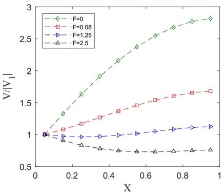
6.5. Numerical Solutions for the Case 3
The viscous flow examples provided in this section of the paper
shed some light on some of the effects of viscosity through the friction
factor. The objective is to estimate the effect of the parameter ![]() on the flow distribution in a
perforated tube with equal-size uniformly distributed holes (10 holes,
on the flow distribution in a
perforated tube with equal-size uniformly distributed holes (10 holes, ![]() ,
, ![]() , and
, and ![]() ).
).
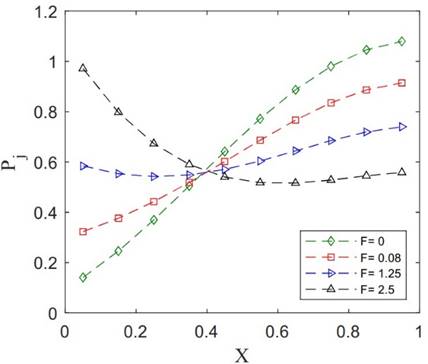
First, let’s assume constant friction factors. Discharged jet
velocities and normalized relative pressure distributions at the holes’
positions are shown in Figure 23 for different values of friction factor.
Figure 23 (a) shows the effect of friction factor on the distribution of jet
velocities. Notice that the highest jet velocities are obtained for ![]() , i.e. ideal flow. Higher values for
, i.e. ideal flow. Higher values for ![]() results
in lower and more uniform jet velocities so that for
results
in lower and more uniform jet velocities so that for ![]() , rather uniform jet velocities are
obtained. Very high values of
, rather uniform jet velocities are
obtained. Very high values of ![]() ,
i.e.
,
i.e. ![]() in this example, results in lower jet
values near the end of the tube. The corresponding pressure distributions are
shown in Figure 23 (b). As expected, while pressure recovery is dominant in the
in this example, results in lower jet
values near the end of the tube. The corresponding pressure distributions are
shown in Figure 23 (b). As expected, while pressure recovery is dominant in the
![]() case, pressure loss due to the
friction is the dominant phenomenon in the
case, pressure loss due to the
friction is the dominant phenomenon in the ![]() case.
case.
Including friction in the flow modeling of real manifolds is crucial for improving prediction accuracy compared to the ideal, frictionless model. Unlike the pressure recovery effect caused by jet discharge, the axial viscous force reduces the pressure buildup along the manifold. Since the local pressure determines the jet outflow, a more accurate pressure prediction leads directly to a more accurate estimation of the lateral flow distribution. In contrast, neglecting friction results in a pressure curve that increases more steeply along the manifold, potentially overestimating jet velocities near the end. This discrepancy becomes more pronounced in long manifolds or when handling more viscous fluids, where friction can become the dominant effect—leading to a decreasing pressure trend, as observed in Figure 23(b).
(a)
(b)
Figure 23. Examples of solutions in Case 3 for constant friction factor. Jet velocities (a) and non-dimensional relative pressures (b).
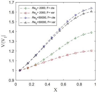
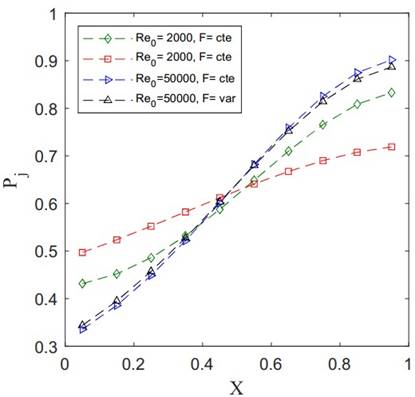
Now, the friction factor is considered a variable quantity. In
this case, the friction factor is a function of the Reynolds number.
Computational results are provided in Figure 24 for both laminar (![]() and turbulent (
and turbulent (![]() flows. The inlet Reynolds number (
flows. The inlet Reynolds number (![]() is defined using
is defined using ![]() (the diameter of the tube) as the
length scale and
(the diameter of the tube) as the
length scale and ![]() as the characteristic velocity.
as the characteristic velocity.
The distributions of jet velocities in these test cases are shown
in Figure 24 (a) and the corresponding pressure distributions are shown in Figure
24 (b). To examine the effect of the variation of ![]() along
the tube on the jet velocity and pressure distribution in both laminar and
turbulent flow examples, results corresponding to the inlet values of
along
the tube on the jet velocity and pressure distribution in both laminar and
turbulent flow examples, results corresponding to the inlet values of ![]() are
also provided and labeled with
are
also provided and labeled with ![]() . Note that both jet velocities and
pressure distribution are more sensitive to the variation of
. Note that both jet velocities and
pressure distribution are more sensitive to the variation of ![]() in
the turbulent flow case.
in
the turbulent flow case.
(a)
(b)
Figure 24. Examples of solutions in Case 3 for variable friction factor. Jet velocities (a) and non-dimensional relative pressures (b).
7. Concluding Remarks
This study presents a computational framework for predicting both inviscid and viscous flow in perforated tube manifold systems. The key contribution of this work lies in the development of a novel, and rather simple, numerical technique that allows engineers to vary both the diameter and spacing of perforations along the tube to achieve a desired flow distribution.
To enhance understanding and simplify the implementation, the method was first applied using ideal (inviscid, incompressible) flow model. This approach not only provides valuable insight into the influence of geometric parameters on flow behavior, but also serves as a reliable initial guess for the more complex viscous flow simulations. Results from the ideal flow model clearly demonstrate the critical role of hole spacing and diameter variation in optimizing flow distribution.
Subsequently, the methodology was extended to viscous flows, incorporating the effects of fluid viscosity through an iterative numerical solution algorithm. Comparison with experimental data shows strong agreement, with a maximum deviation of less than 10%, thereby validating the accuracy of the viscous model.
Additionally, a general mathematical framework capable of representing a wide range of geometrical and physical complexities in perforated manifolds has been formulated. The solution strategy for this extended model will be the focus of future work.
To wrap up the paper, it is very informative, and practically useful, to examine the range of the validity and applicability of the ideal flow model before making a few comments about the viscosity effects in this last section of the paper.
7.1. Limitations of the Ideal Flow Model
To discuss the range of the validity of the ideal flow model, it
is very useful to first show the extent to which the ideal flow results comply
with the predictions of viscous flow models. In Figure 25, a comparison has
been made using the viscous flow results provided by Wang [23]. In the viscous
flow results from [23], only the effect of friction is considered, and ideal
discharge from the holes is assumed. It is clear that the semi-analytical ideal
flow results in this case, in which ![]() , are qualitatively relevant and
rather close to the viscous flow results (maximum error around 20%). The
pressure drop due to the viscosity effects is observed in Figure 25. Note that
the Euler number (
, are qualitatively relevant and
rather close to the viscous flow results (maximum error around 20%). The
pressure drop due to the viscosity effects is observed in Figure 25. Note that
the Euler number (![]() ) is reported in [23]. Also,
) is reported in [23]. Also, ![]() , mentioned in Figure 25, represents
the
, mentioned in Figure 25, represents
the ![]() ratio
and
ratio
and ![]() represents the Reynolds number.
represents the Reynolds number.
Figure 25. Comparison of ideal and viscous flow results in a perforated tube.
Further studies using the ideal flow model show that the solutions
are not physically justified for Λ values greater than π/2. In fact, for ![]() values greater than 1.57, the holes
near the inlet suck the fluid instead of discharging it. Furthermore, lack of viscosity
makes it possible for the fluid to go through strange maneuvers like the one
shown in Figure 26 for
values greater than 1.57, the holes
near the inlet suck the fluid instead of discharging it. Furthermore, lack of viscosity
makes it possible for the fluid to go through strange maneuvers like the one
shown in Figure 26 for ![]() . It is well known that the ideal flow
models may predict unrealistic flow accelerations/decelerations and/or sudden
changes in the flow direction. Consecutive negative and positive axial
velocities in a tube, as shown in Figure 26, are not practically feasible.
Therefore, care should be taken whenever an ideal flow model is used to analyze
or predict the flow distribution in perforated tubes. Here, we recommend the
. It is well known that the ideal flow
models may predict unrealistic flow accelerations/decelerations and/or sudden
changes in the flow direction. Consecutive negative and positive axial
velocities in a tube, as shown in Figure 26, are not practically feasible.
Therefore, care should be taken whenever an ideal flow model is used to analyze
or predict the flow distribution in perforated tubes. Here, we recommend the ![]() value
as a guide in this regard.
value
as a guide in this regard.
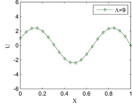
Figure 26. An example of an unrealistic ideal flow solution.
Ideal flow model is an
attractive choice for the rough and initial evaluation of the effects of the
geometrical parameters. As discussed thoroughly, for the class of perforated
tubes shown schematically in Figure 1, the important geometrical parameters are
![]() and
and ![]() . This means that for a given tube (
. This means that for a given tube (![]() and
and
![]() fixed), the only design parameters
are the spacing or pitch (
fixed), the only design parameters
are the spacing or pitch (![]() )
and diameter (
)
and diameter (![]() of the holes. When
of the holes. When ![]() and/or
and/or
![]() vary
arbitrarily along the tube, analytical solution of the governing equation for
the velocity field along the tube becomes prohibitively difficult and the
numerical recipe prescribed in this paper provides a handy computational tool.
vary
arbitrarily along the tube, analytical solution of the governing equation for
the velocity field along the tube becomes prohibitively difficult and the
numerical recipe prescribed in this paper provides a handy computational tool.
7.2. Comments on the viscous flow results
Complex physical phenomena occur in a perforated tube carrying a viscous fluid. Pressure loss due to the fluid friction, losses associated with the flow across a hole, including the vena-contracta phenomenon, and pressure recovery when the fluid passes over a hole in a tube are all real flow effects that are very difficult to model accurately. In the viscous flow results in this paper, the skin friction is taken into consideration and the pressure recovery is considered for a simple case in which the discharged jets are exactly normal to the axis of the tube. Results show that the pressure distribution in the tube, which ultimately controls the distribution of jet velocities, is governed by two conflicting factors: pressure drop due to the friction and pressure rise due to the pressure recovery.
Further studies have been carried out to include more real flow phenomena in the mathematical model and to take into consideration simultaneous effects of the physical and geometrical parameters on the flow through perforated tubes. Discussions regarding solution strategies and results for these more complicated cases are beyond the scope of the present paper.
References
[1]S. K. Jain, K. K. Singh, and R. P. Singh, “Microirrigation Lateral Design Using Lateral Discharge Equation,” Journal of Irrigation and Drainage Engineering, vol. 128, no. 2, pp. 125–128, 2002. View Article
[2] R. P. Perold, “Computer Design of Microirrigation Pipe Systems,” Journal of the Irrigation and Drainage Division, vol. 105, no. 4, pp. 403–417, Dec. 1979. View Article
[3] S. Qvist and E. Bubelis, “Passive Shutdown Systems for Fast Neutron Reactors,” International Atomic Energy Agency, 2020
[4] S. A. Bhardwaj, “Tarapur Atomic Power Project-3&4: Design Innovations,” An International Journal of Nuclear Power, vol. 19, pp. 1–4, 2005.
[5] A. V. Kulkarni, “Design of a Pipe/Ring Type of Sparger for a Bubble Column Reactor,” Chemical Engineering & Technology: Industrial Chemistry‐Plant Equipment‐Process Engineering‐Biotechnology, vol. 33, no. 6, pp. 1015–1022, 2010. View Article
[6] A. V. Kulkarni and J. B. Joshi, “Design and Selection of Sparger for Bubble Column Reactor. Part II: Optimum sparger type and design,” Chemical Engineering Research and Design, vol. 89, no. 10, pp. 1986–1995, 2011. View Article
[7] C. N. Wang, “A Numerical Scheme for The Analysis of Perforated Intruding Tube Muffler Components,” Applied Acoustics, vol. 44, no. 3, pp. 275–286, 1995. View Article
[8] D. Neihguk, M. L. Munjal, and A. Prasad, “Pressure Drop Characteristics of Perforated Pipes with Particular Application to the Concentric Tube Resonator,” SAE Technical Papers, vol. 2015-June, 2015. View Article
[9] A. Andreini, R. Da Soghe, B. Facchini, F. Maiuolo, L. Tarchi, and D. Coutandin, “Experimental and Numerical Analysis of Multiple Impingement Jet Arrays for an Active Clearance Control System,” Journal of Turbomachinery, vol. 135, no. 3, pp. 1–9, 2013. View Article
[10] R. DaSoghe, L. Mazzei, L. Tarchi, L. Cocchi, A. Picchi, B. Facchini, L. Descamps, J. Girardeau and M. Simon,“Development of Experimental and Numerical Methods for the Analysis of Active Clearance Control Systems,” Journal of Engineering for Gas Turbines and Power, 2020. View Article
[11] A. Tomor and G. Kristóf, “Validation of a Discrete Model for Flow Distribution in Dividing-Flow Manifolds: Numerical And Experimental Studies,” Periodica Polytechnica Mechanical Engineering, vol. 60, no. 1, pp. 41–49, 2016. View Article
[12] T. Afrin, N. B. Kaye, A. A. Khan, and F. Y. Testik, “Parametric Study of Perforated Pipe Underdrains Surrounded by Loose Aggregate,” Journal of Hydraulic Engineering, vol. 142, no. 12, p. 04016066, 2016. View Article
[13] M. T. Dhotre and J. B. Joshi, “Design of a Gas Distributor: Three-dimensional CFD Simulation of a Coupled System Consisting of a Gas Chamber and a Bubble Column,” Chemical Engineering Journal, vol. 125, no. 3, pp. 149–163, 2007. View Article
[14] F. Ben Ahmed, R. Tucholke, B. Weigand, and K. Meier, “Numerical Investigation of Heat Transfer and Pressure Drop Charactristics for Different Hole Geometries of a Turbine Casing Impingement Cooling System,” In Turbo Expo: Power for Land, Sea, and Air, vol. 54655, pp. 1095-1108. 2011 View Article
[15] A. W. Chen and E. M. Sparrow, “Journal of Engineering for Gas Turbines and Power,” Appl Therm Eng, vol. 29, no. 13, pp. 2689–2692, 2009. View Article
[16] J. Yang, K. Cheng, K. Zhang, C. Huang, and X. Huai, “Numerical Study on Thermal and Hydraulic Performances of a Hybrid Manifold Microchannel with Bifurcations for Electronics Cooling,” Applied Thermal Engineering, vol. 232, 2023. View Article
[17] D. E. Guerfi, S. Roux, N. Allanic, A. Sarda, and D. Lecointe, “Parametric Study on Enhanced Thermal Management via Regulated Impingement Boiling Cooling,” Journal of Fluid Flow, Heat and Mass Transfer (JFFHMT), vol. 11, pp. 145–157, Jun. 2024. View Article
[18] R. Da Soghe and C. Bianchini, “Aero-Thermal Investigation of Convective and Radiative Heat Transfer on Active Clearance Control Manifolds,” in Proceedings of ASME Turbo Expo 2019: Turbomachinery Technical Conference and Exposition GT2019, pp. 1–10, 2019, View Article
[19] S. Pachpute and B. Premachandran, “Turbulent Multi-jet Impingement Cooling of a Heated Circular Cylinder,” International Journal of Thermal Sciences, vol. 148, p. 106167, 2020. View Article
[20] G. Kogekar and R. J. Kee, “Model-based Performance for Gas Distribution from Perforated Manifolds and Spargers,” Chemical Engineering and Processing - Process Intensification, vol. 140, no. April, pp. 127–135, 2019. View Article
[21] J. Wang, “Theory of Flow Distribution in Manifolds,” Chemical Engineering Journal, vol. 168, no. 3, pp. 1331–1345, 2011. View Article
[22] F. LU, Y. hao LUO, and S. ming YANG, “Analytical and Experimental Investigation of Flow Distribution in Manifolds for Heat Exchangers,” Journal of Hydrodynamics, vol. 20, no. 2, pp. 179–185, 2008. View Article
[23] J. Wang, Z. Gao, G. Gan, and D. Wu, “Analytical Solution of Flow Coefficients for A Uniformly Distributed Porous Channel,” Chemical Engineering Journal, vol. 84, no. 1, pp. 1–6, 2001. View Article
[24] M. K. Bassiouny and H. Martin, “Flow Distribution and Pressure Drop in Plate Heat Exchangers, I U-type Arrangement,” Chemical Engineering Science, vol. 39, no. 4, pp. 693–700, 1984. View Article
[25] R. A. Bajura, “A Model for Flow Distribution in Manifolds,” Journal of Engineering for Power, vol. 93, no. 1, pp. 7–12, 1971. View Article
[26] A. Acrivos, B. D. Babcock, and R. L. Pigfords, “Flow Distributions in Manifolds,” Chemical Engineering Science, vol. 10, pp. 112–124, 1959. View Article
[27] H. Liu, Q. Zong, H. Lv, and J. Jin, “Analytical Equation for Outflow Along the Flow in A Perforated Fluid Distribution Pipe,” PLoS One, vol. 12, no. 10, pp. 9–19, 2017. View Article
[28] L. Czetany, Z. Szantho, and P. Lang, “Rectangular Supply Ducts with Varying Cross Section Providing Uniform Air Distribution,” Applied thermal engineering, vol. 115, pp. 141–151, 2017. View Article
[29] J. Wang and H. Wang, “Discrete Method for Design of Flow Distribution in Manifolds,” Applied thermal engineering, vol. 89, pp. 927–945, 2015. View Article
[30] M. M. Rahman and A. Bénard, “Model for Flow and Pressure Distribution in Tapered Headers Of U-type Plate Heat Exchangers,” Applied thermal engineering, vol. 249, 2024. View Article
[31] J. Wang, G. H. Priestman, and D. Wu, “A Theoretical Model of Uniform Flow Distribution for The Admission of High-energy Fluids to A Surface Steam Condenser,” Journal of Engineering for Gas Turbines and Power, vol. 123, no. 2, pp. 472–475, 2001. View Article
[32] R. K. Singh and A. Rama Rao, “Simplified Theory for Flow Pattern Prediction in Perforated Tubes,” Nuclear Engineering and Design, vol. 239, no. 10, pp. 1725–1732, 2009. View Article
[33] A. V. Kulkarni, S. S. Roy, and J. B. Joshi, “Pressure and Flow Distribution in Pipe and Ring Spargers: Experimental Measurements and CFD Simulation,” Chemical Engineering Journal, vol. 133, no. 1–3, pp. 173–186, 2007. View Article