Journal of Fluid Flow, Heat and Mass Transfer (JFFHMT)

ISSN: 2368-6111

Study on Reducing the Order of Mathematical Model for Combustion Instability

Koji Maeta¹, Takenao Ohkawa¹

¹Graduate School of System Informatics, Kobe University
1-1 Rokkodai-Cho Nada-Ku Kobe-City, Hyogo 657-8501, Japan
189x601x@stu.kobe-u.ac.jp;
ohkawa@kobe-u.ac.jp

Abstract - This study proposes a low-dimensional thermoacoustic model for predicting pressure fluctuations in lean-burn combustion systems. Traditional monitoring approaches based solely on experimental data or physical models lack accuracy and responsiveness for real-time applications. To address this limitation, a linearized acoustic wave equation incorporating heat release fluctuations and flow-induced acoustic sources was formulated using conservation laws. A finite element Analysis (FEA) model was developed and implemented in the time domain via the Newmark-β scheme. A simplified Rijke tube model was constructed, with input data such as temperature distribution derived from high-speed flame image analysis, enabling computational efficiency and near-real-time prediction without CFD. Experimental validation was conducted with a premixed combustor under various air flow rates and burner positions. The predicted and observed pressure signals showed increasing amplitude with leaner mixtures. The correlation coefficients for the peak frequencies of the first and second modes were 0.77 and 0.67, respectively. Damping ratios estimated using Hilbert transform and curve fitting yielded a correlation coefficient of 0.73. The most unstable flame location corresponded to the position of maximum acoustic pressure gradient, consistent with the theoretical forcing term formulation. These results demonstrate the model’s capability to capture combustion instability trends and its potential for future integration with data assimilation and machine learning techniques.

Keywords: Combustion instability, Mathematical Model, Low-dimensional model, Data Assimilation, Finite Element Method

© Copyright 2025 Authors - This is an Open Access article published under the Creative Commons Attribution License terms Creative Commons Attribution License terms. Unrestricted use, distribution, and reproduction in any medium are permitted, provided the original work is properly cited.

Date Received: 2025-04-06
Date Revised: 2025-04-28
Date Accepted: 2025-05-01
Date Published: 2025-05-05

1. Introduction

In recent years, the demand for more efficient and safer operation of industrial systems has underscored the urgent need to advance health monitoring technologies for combustion devices. Traditional monitoring approaches have relied solely on either observational data or physics-based mathematical models; however, these methods, when used independently, are often inadequate—particularly for real-time state estimation and anomaly detection. To address these limitations, data assimilation techniques that combine observational data with mathematical models have garnered increasing attention [1] – [3]. The objective of this study is to develop a low-dimensional thermoacoustic model capable of real-time prediction and to lay the groundwork for its future integration with data assimilation frameworks. Data assimilation not only enhances the accuracy of model-based predictions but also enables real-time estimation of system states, providing significant advantages for the control of combustion devices and prompt response to abnormal operating conditions. These benefits can lead to improved operational efficiency, enhanced safety, and prolonged equipment lifespan. Furthermore, data assimilation enables estimations that account for subtle variations and nonlinear behaviors often neglected by conventional models, thereby deepening the understanding of complex combustion phenomena. Nóvoa, Noiray, Dawson, and Magri [4] demonstrated the potential of real-time monitoring by developing a digital twin of thermoacoustic instabilities, employing Kalman filtering to estimate the dynamic evolution of azimuthal combustion oscillations. Sarkar et al. [5] introduced a data assimilation-based prediction framework for combustion instabilities in a laboratory-scale combustor, achieving high-accuracy predictions through the integration of sensor measurements and model data. In a related effort, Banaszuk, Ariyur, Krstić, and Jacobson [6] proposed an adaptive control algorithm to suppress combustion instabilities in gas turbine engines by combining an extended Kalman filter-based frequency estimator with a phase-shift controller to modulate fuel injection in real time.

In this study, we focus on the pressure fluctuations in combustion devices and aim to construct a low-dimensional model, rapid predictions can be achieved with reduced computational cost, and, in the future, by integrate this model with data assimilation methods, we aim to build a more accurate and efficient framework for real-time state estimation and prediction. Therefore, to predict and analyze combustion-induced pressure fluctuations, it is essential to first formulate the governing thermoacoustic system, as described in the following section.

2. Formulation of Thermoacoustic Systems

Combustion instabilities in internal combustion engines are considered self-excited oscillations that form a feedback loop, as shown in Figure 2.1. Figure 2.1 schematically illustrates the feedback loop between combustion-induced pressure fluctuations and fuel concentration oscillations, which is fundamental to thermoacoustic instability. The combustion inside the internal combustion engine generates acoustic oscillations due to the repeated expansion and contraction of the gas, which induces fluctuations in the fuel concentration within the nozzle. These fuel concentration fluctuations propagate downstream with the flow and, upon combustion, generate pressure fluctuations.

In this chapter, we examine a mathematical model for the feedback loop that encompasses these physical phenomena.

To model the dynamics of combustion and acoustics, we define the fundamental equations based on fluid dynamics, as shown in Eq.1 to Eq.4. Eq.1 presents the mass conservation low, which governs the inflow and outflow of fluid. Here, we assume that mass variation due to sources or sinks, such as fluid injection or suction, is not considered. Eq.2 is the equation of motion, which describes the force balance. It is derived from the equilibrium between the pressure acting on a boundary surface and the inertial force. Eq.3 is the heat transport equation, which expresses the conservation of heat in the combustion region. It is assumed that the fluid undergoes heat changes only within the combustion zone, while all other regions are considered adiabatic. Eq.4 is the equation of state, which describes the relationship between temperature variations and energy changes.

Where ρ is Density, t is Time, u is Flow velocity, p is Pressure fluctuation, φ is Viscous and external force, T is Temperature, S is Entropy, q is Heat release density, c is Speed of sound, γ is Specific heat ratio, D/Dt denotes Lagrange derivative. In this paper, we focus on the trajectory of a specific fluid particle in a system with a steady flow, as shown in Figure 2.1. Therefore, we introduce the concept of the Lagrange derivative, which is used when observing particle trajectories in a fixed spatial coordinate system. By substituting Eq.3 into Eq.4, we obtain Eq.5

(1)

(2)

(3)

(4)

(5)

By rearranging the terms related to the flow velocity in the Lagrange derivative of Eq.5 and substituting Eq.1 and Eq.2, the nonlinear acoustic wave equation can be expressed as Eq.6. Eq.6 represents the nonlinear acoustic wave equation, integrating flow- induced and combustion-induced source terms to model self-excited oscillations.

(6)

Dowling [7] and Hedge at al. [8] considered the phenomenon using a wave equation that accounts only for the heat source term generated by combustion, which appears as the first term on the right-hand side.

In this paper, we extend the formulation by also considering the source term due to small velocity fluctuations indued by the flow, based on the approach of Ikeda [9]. This second term is considered equivalent to the source term arising from fluid noise, as defined in the field of aeroacoustics by Klein et al. [10] and Toquard et al. [11]. The terms from the fourth and beyond containing (∇∙u)X', represent the source terms associated with flow divergence. Since this paper does not assume a system with external aerodynamic source terms, these terms are also excluded from the formulation. Focusing on the fluctuating components of various physical quantities, we derive the linearized wave equation, which is presented as Eq.7.

(7)

Here, to improve the clarity of the solution, we express the entropy and temperature in terms of pressure and density in Eq.7. The linearized equation of motion and the equation of state are then defined as Eq.8 and Eq.9, respectively. By substituting Eq.8 and Eq.9 into Eq.7 and rearranging the terms, we finally obtain Eq.10.

(8)

(9)

(10)

Here, Crocco et al. [12]-[13] and Culick et al. [14] have proposed Eq.11, which relates the fluctuations of the premixed gas inside the fuel nozzle to the combustion state of the advected gas.

(11)

Where v is Flow velocity of the premixed gas, w is Fuel density consumption rate due to chemical reactions, τ is Advection time of fuel concentration fluctuations from the fuel nozzle tip to the flame position. Based on this relationship Eq.12 and Eq.13, by defining , , Eq.10 can be rewritten in the form of Eq.14. To numerically solve the derived thermoacoustic wave equations and simulate pressure fluctuations, the following section introduces a finite element method based analytical approach.

(12)

(13)

(14)

2.1. Finite Element Analysis (FEA)

This study investigates finite element analysis that contributes to real-time prediction through data assimilation. When the thermoacoustic phenomenon is simplified as a one-dimensional model in the flow direction, it can be expressed by Eq.15.

(15)

To express the second-order spatial differential equation in a first-order form, Eq.15 is converted into a weak form. By multiplying by an arbitrary function φ with respect to x and integrating over the spatial domain, and then performing integration by parts on the second term, the equation can be written as Eq.16. Eq.16 reformulates the governing equation into a weak form suitable for finite element discretization, allowing for numerical implementation.

(16)

Discretization is performed. The physical quantities at each node are defined as shown in Eq.17

(17)

Where i represents an arbitrary node, i denotes the total number of nodes, and N is the basis function. Substituting Eq.17 into Eq.16, the first term of Eq.16 can be expressed as shown in Eq.18. The second term can be neglected because both ends of the flow path are acoustically open, resulting in p^'=0.

(18)

Where m_ij=∫N_i(x)N_j(x)dx. The second term can be neglected because both ends of the flow path are acoustically open, resulting in p^'=0. The third term can be expressed as shown in Eq.19

(19)

Where K_ij=c²∫N'_i(x)N'_j(x)dx. The fourth term can be expressed as shown in Eq.20.

(20)

Where . The fifth term can be written in the same way as the fourth term, as shown in Eq.21.

(21)

Where . The sixth term can be written in the same way as Eq.22 and Eq.23.

(22)

(23)

Where . Thus, by substituting Eq.18 to Eq.23 into Eq.16, the following expression is obtained.

(24)

Here, since φ is an arbitrary function, for Eq.24 to hold, it must satisfy the condition given by Eq.25. Eq.25 ensures that the discretized system satisfies the weak form for arbitrary test functions, leading to the FEA formulation for acoustic pressure evolution.

(25)

Using Eq.25, a time history analysis is performed with the acoustic FEA. The time evolution is solved using the Newmark- β method, as shown Eq.26. Eq.26 applies the Newmark- β method to solve the time-dependent system, balancing stability and accuracy for transient thermoacoustic simulations.

(26)

Where p'_i. represents the unknown sound pressure level at time t, while p'_i-t represents the known sound pressure at time t-τ. The relationship between the step number and time is given by t=∆t(i) and τ=∆tT. Expressing the current p'_i in terms of the previous step p'_i-1, it can be written as Eq.27 and Eq.28.

(27)

(28)

From the relationship between the two equations above and Eq.26, Eq.29 is ultimately derived. Based on the FEA formulation, we constructed a computational model, which is presented in the next section.

(29)

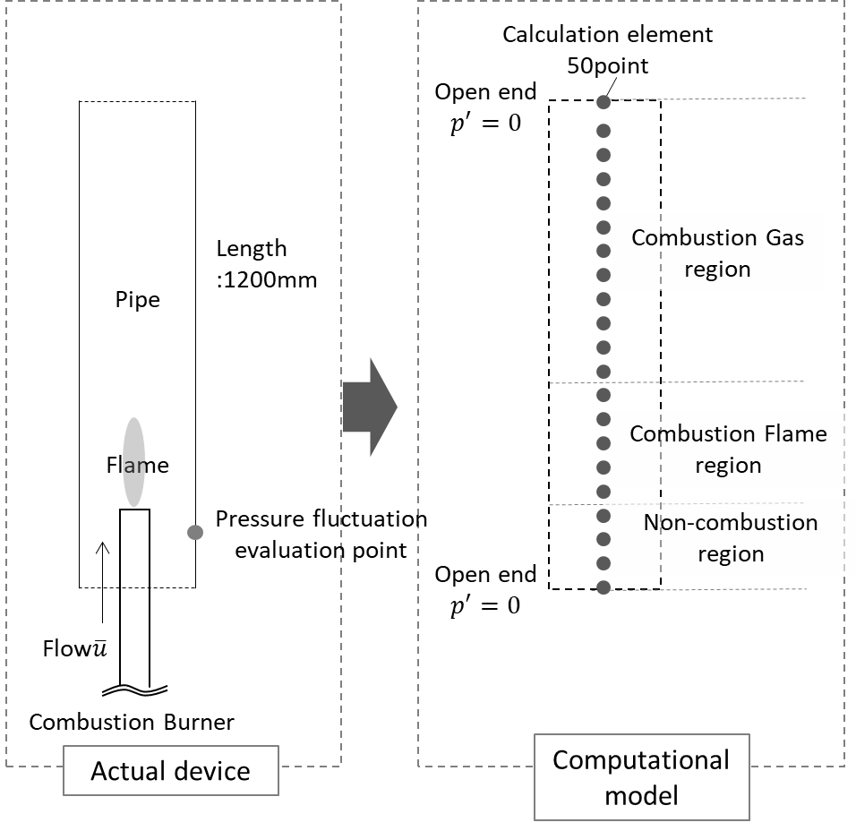
2.2. Computational model

The computational model is shown in Figure 2.2. Figure 2.2 shows the simplified Rijke-tube inspired configuration adopted for numerical simulations, focusing on essential features of thermoacoustic feedback while maintaining computational efficiency. A heat source (Combustion burner) is placed inside a cylindrical tube, and the pressure fluctuations occurring within the tube are computed. The computational model employs the FEA described in Chapter2.1, with a total length of 1200mm divided into 50 computational elements.

The computational input was set based on the method shown in Table 2.1. Table2.1 lists the FEA input parameters, derived from flame imaging data to enable real-time capable, experimentally anchored pressure fluctuation predictions. The input for the FEA in this study was determined from flame image data captured using a high-speed camera, as described in Section 3.1. Specifically, the spatial distribution of temperature data was estimated based on the relationship between discretely measured temperature data and combustion image data, and various physical properties and state variables were calculated from the gas composition and temperature information.

The first reason for employing this method is that, in the condition monitoring of industrial products assumed in this study, it is possible to acquire real-time combustion flame image data inside an internal combustion engine. The second reason is that state variable prediction considering chemical reactions, combustion processes, and fluid dynamics, such as combustion CFD, requires a significant amount of computational time, making it unsuitable for real-time prediction of pressure fluctuation levels.

In this study, the input data for future physical properties and state variables required to compute the desired pressure fluctuation levels were derived from computational input data based on experimentally captured image data. As a future research direction, we aim to apply data analysis techniques such as machine learning and deep learning to predict the necessary future input data based on operational parameters related to fuel supply and historical combustion flame image data. To validate the computational model and assess its predictive capability, an experimental study was conducted, as described in the following section.

3. Experiment summary

3.1. Experimental Device and Measuring Equipment

The experimental device used in this study is shown in Figure 3.1. In this experiment, a premixing nozzle equipped with a swirler was inserted into a rectangular cylinder with a base dimension of 50mm square and a length of 1200mm. Liquefied petroleum (LP) gas (main component: propane) and air were supplied to the nozzle using a mass flow meter. The combustion oscillation level was measured using a pressure fluctuation level sensor installed upstream of the combustion cylinder. This microphone can measure sound pressure levels of 30dB (10^-3Pa) in the 4-70kHz range. As shown in Figure 5.1(Mentioned later), the maximum sound pressure level was defined as 148dB(410Pa) with a normalized sound pressure level of 1. Therefore, it is possible to measure a Normalized sound pressure level of 10^-5 or less. As shown in Figure 5.1, the average value of the normalized sound pressure level under operating conditions with low combustion oscillation levels is on the order of 10^-2. It can be said that this experiment has sufficient measurement accuracy.

The experimental apparatus used in this study was equipped with a visualization window to observe the flame inside the combustor. Flame images were captured using a high-speed camera through this visualization window. Simultaneously, the temperature measured by a thermocouple sensor was correlated with the flame images to estimate the temperature distribution inside the combustor.

The relative position of the acoustic mode generated inside the combustor and the heat release concentration of the flame is a crucial factor in evaluating combustion instability. In this experiment, to intentionally vary the relative position of the flame with respect to the acoustic mode inside the combustor, the visualization window was designed to be relocatable in the flow direction.

3.2. Experimental Conditions

When obtaining the data under various combustion conditions, the combustion oscillation level and flame image data were obtained by keeping the LP gas flow constant while changing the air flow condition step by step as shown in Table 3.1.

The maximum air flow rate was set to the limit conditions for flame lift and blowout, while the gas flow rate was set to the maximum allowable value considering the heat resistance of the nozzle(uncooled). As shown on the left of Figure 3.2, the nozzle was positioned at L/2, L/4, and L/8 from the bottom(upstream) end of the combustion cylinder, relative to the total length of the cylinder(L). This is because the relative position between the flame and the antinode or node of the first-order acoustic mode is believed to influence the level of combustion instability. The air flow rate was set to vary step by step, as shown in right of Figure 3.2.

4. Guidelines for evaluations

4.1. Damping ratio

The method for estimating the damping ratio, a key parameter in evaluating vibration characteristics, is described herein. As a first step, the Hilbert transform was performed in accordance with the definition provided in Eq.30 to extract the envelope of the vibration waveform.

(30)

Where x(t) is a real-valued function. is the Hilbert transform of a real-valued function."*" denotes convolution, and the integral represents the Cauchy principal value. Based on the result above, the envelope and slope of the vibration waveform can be expressed as shown in Eq.31 and Eq.32.

(31)

(32)

Based on Eq.32, the logarithmic decrement and the damping ratio at the natural frequency are formulated as Eq.33 and Eq.34, respectively.

(33)

(34)

Where δ denotes the logarithmic decrement, f_n is the natural frequency, and ζ represents the damping ratio.

5. Results and Discussion

An example of the time history waveform of the observed pressure fluctuation level, measured using the combustion system and instrumentation described in Chapter 3, is shown in Figure5.1. An example of the predicted time history waveform, calculated using the thermoacoustic FEA model described in Chapter 2, is shown in Figure 5.2.

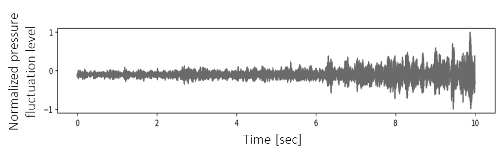
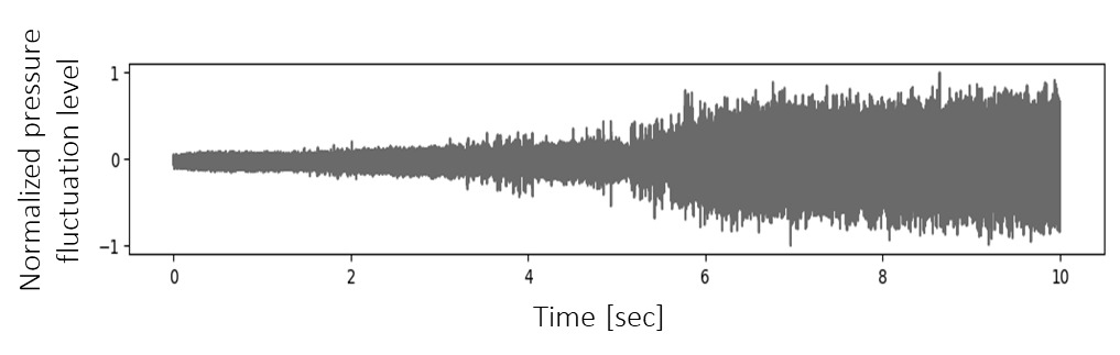
From Figures 5.1 and 5.2, it was confirmed that both the observed and predicted results exhibit a trend of increasing amplitude levels as the air-to-fuel ratio is incrementally increased under the lean combustion conditions described in Section 3.2.

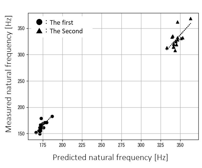
Figure 5.3 presents a comparison of the first and second peak frequencies obtained from the FFT analysis of all cases for both observed and predicted results. The horizontal axis represents the predicted values, while the vertical axis represents the observed values. The correlation coefficients for the first and second modes were found to be 0.77 and 0.67, respectively, indicating a reasonable agreement between the two.

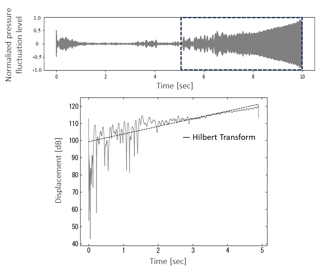
Subsequently, curve fitting was applied to the amplitude envelope of the vibration signal, which was calculated using the Hilbert Transform as described in Chapter 4, to estimate the logarithmic decrement and damping ratio (Figure 5.4). The data interval used for curve fitting was set between 5 and 10 seconds, during which the vibration amplitude increased, as indicated in Figure 5.4.

For all observed and predicted cases, the damping ratio was calculated for the dominant response mode, defined as the peak response below 500Hz (first or second mode). The results are presented in Figure 5.5. The vertical axis represents the observed values, while the horizontal axis represents the predicted values. The correlation coefficient between the two was found to be 0.73, indicating a generally consistent trend. These results demonstrate that the proposed analytical model is capable of reproducing the trend of combustion instability.

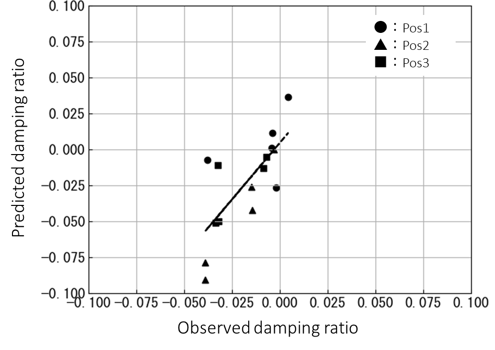
From the results shown in Figure 5.5, it was found that the flame position exhibiting the strongest tendency toward instability—characterized by significantly negative damping ratios in both observed and predicted cases—was Pos2. This location corresponds to the point where the pressure gradient (∇p'(t)) of the first open-open acoustic mode reaches its maximum. As described by Eq.14 in Chapter 2, the external forcing term is expressed as the product of the mode-induced pressure gradient (∇p'(t)) and the mean heat release rate (q ̅). The increase in this forcing term at Pos2 suggests a possible mechanism for the enhanced combustion instability observed at this position.

5. Conclusion

In this study, a low-dimensional thermoacoustic model was developed and validated for predicting pressure fluctuation behavior in combustion devices operating under lean burn conditions. By integrating a finite element formulation with experimentally derived input data, the model was capable of simulating the time evolution of pressure fluctuations and capturing the dominant frequency components associated with combustion instability.

The predicted results demonstrated good agreement with experimental observations, as evidenced by the correlation coefficients of 0.77 and 0.67 for the first and second mode peak frequencies, respectively. Furthermore, damping ratios estimated via Hilbert transform and curve fitting techniques showed a correlation coefficient of 0.73 between predicted and observed values, indicating that the proposed model effectively captures the instability characteristics of the system.

A detailed analysis revealed that the most unstable flame position corresponded Pos2, where the pressure gradient of the first acoustic mode was maximized. This finding is consistent with theoretical predictions, which suggests that the external forcing term—defined as the product of the pressure gradient and the mean heat release rate—plays a critical role in driving combustion instability.

These results confirm the validity of the proposed modelling approach and its potential applicability to real-time monitoring and control of combustion systems. Nevertheless, it should be noted that this study assumes steady-state flow conditions and neglects external aerodynamic noise sources. Although these simplifications enable efficient modelling and real-time prediction, they may limit the model’s applicability under conditions involving significant flow unsteadiness or external acoustic disturbances. To address these limitations, future research will focus on incorporating more complex flow dynamics and external forcing effects, as well as enhancing the real-time predictive capabilities through the integration of data assimilation techniques and machine learning-based estimation of input parameters.

References

[1] R. Daley, Atmospheric Data Analysis. Cambridge, UK: Cambridge University Press, 1991.
[2] M. Asch, M. Bocquet, and M. Nodet, Data Assimilation: Methods, Algorithms, and Applications. Philadelphia, PA: SIAM, 2016. View Article
[3] K. Law, A. Stuart, and K. Zygalakis, Data Assimilation: A Mathematical Introduction. New York, NY: Springer, 2015. View Article
[4] A. Nóvoa, N. Noiray, J. R. Dawson, and L. Magri, "A real-time digital twin of azimuthal thermoacoustic instabilities," J. Fluid Mech., vol. 1001, Art. no. A29, 2024. View Article
[5] S. Sarkar, S. R. Chakravarthy, V. Ramanan, and A. Ray, "Dynamic data-driven prediction of instability in a swirl-stabilized combustor," International Journal of Spray and Combustion Dynamics, vol. 8, no. 4, pp. 235-253, 2016. View Article
[6] A. Banaszuk, K. B. Ariyur, M. Krstić, and C. A. Jacobson, "An adaptive algorithm for control of combustion instability," Automatica, vol. 40, no. 11, pp. 1965-1972, 2004. View Article
[7] A. P. Dowling, "The Calculation of Thermoacoustic Oscillations," J. Sound Vib., vol. 180, no. 4, pp. 557-581, 1995. View Article
[8] U. Hegde, D. Reuter, and B. T. Zinn, "Sound Generation by Ducted Flames," AIAA J., vol. 26, no. 5, pp. 532-537, 1988. View Article
[9] K. Ikeda, "Linear Instability Analysis of Lean Premixed Combustion," J. Therm. Sci. Technol., vol. 7, no. 4, pp. 649-664, 2012. View Article
[10] S. A. Klein and J. B. W. Kok, "Sound Generation of Turbulent Non-Premixed Flames," Combust. Sci. Technol., vol. 149, pp. 267-295, 1999. View Article
[11] L. Crocco and S. I. Cheng, Theory of Combustion Instability in Liquid Propellant Rocket Motors. London: Butterworths Scientific Publication, 1956. View Article
[12] L. Crocco, "Research on Combustion Instability in Liquid Propellant Rockets," Proc. Combust. Inst., vol. 12, pp. 85-99, 1968. View Article
[13] F. E. C. Culick and V. Yang, "Overview of Combustion Instabilities in Liquid-Propellant Rocket Engines," Prog. Astronaut. Aeronaut., vol. 169, pp. 3-37, 1995. View Article