Journal of Fluid Flow, Heat and Mass Transfer (JFFHMT)
ISSN: 2368-6111

Volume 11 - Year 2024 - Pages 296-310
DOI: 10.11159/jffhmt.2024.030
A Theoretical Study of a Micro-Channel Pressure-Driven Flow of Electrically Conducting Liquids in the Presence of a Transversal Magnetic Field
Érick Marcelino Miranda1, Marcos Fabrício de Souza Aleixo Filho1, Francisco Ricardo Cunha 1
1University of Brasilia, Faculty of Technology, Department of Mechanical Engineering, Fluid Mechanics of Complex Flows Group - VORTEX
Brasilia, Brazil
erick99marcelino@outlook.com; mffilhoaleixo@gmail.com; frcunha@unb.br
Abstract - This work examines the effects of a transversal and uniform magnetic field on an electrically conducting liquid. The bottom wall is porous and therefore penetrable, where the jump of shear stress is given in terms of a suitable relative velocity by a semi-empirical boundary condition. The formulation of the flow problem is based on the incompressible Magnetohydrodynamics (MHD) governing equations in terms of non-dimensional variables. The relevant physical parameter measuring the relative importance between magnetic and viscous forces is identified as the Hartmann number. The solution of the problem shows the existence of a flow deceleration strongly dependent upon the Hartmann number. In addition, another interesting result is a decrease in the magnitude of the longitudinal component of the magnetic flux density as Hartmann number increases. The application of a transverse magnetic field in the flow of an electrically conducting fluid in tiny pores can produce an effective effect like the flow deceleration produced as the porous medium permeability is decreased. Therefore, it seems to be possible to produce such an effect by just monitoring the magnetic field instead of changing the complex microstructure of a porous medium. Exact and asymptotic solutions are obtained for the velocity and pressure fields of the unidirectional channel flow. The asymptotic solution describes very well the physical behavior of the flow for Hartmann less than unit. In addition, using the asymptotic solutions is possible to split the flow solution in two parts: a purely hydrodynamic contribution and a leading order magnetic contribution in terms of the Hartmann number.
Keywords: Channel Flow, Penetrable Boundary, Magnetic Field, Flow Control.
© Copyright 2024 Authors - This is an Open Access article published under the Creative Commons Attribution License terms. Unrestricted use, distribution, and reproduction in any medium are permitted, provided the original work is properly cited.
Date Received: 2024-01-24
Date Revised: 2024-07-25
Date Accepted: 2024-08-15
Date Published: 2024-09-30
1. Introduction
Magnetohydrodynamics (MHD) studies the interaction between an electrically conducting fluid (non-magnetic) and a magnetic field. Flows with MHD effects are a part of fluid mechanics involving these fluids (such as salted water, ionized gases, or liquid metal) and a magnetic field [1]. The industry has used this flow type in several applications, including convection inhibition, mixing [2], heating [3], deceleration [4], and fluid pumping. The laminar channel flow with a porous wall was already studied experimentally by Beavers and Joseph [5] and analytically using an extension of the Darcy law with a quadratic term in velocity by Cunha [6].
The central governing equation in the MHD problem is the modified Navier-Stokes (with the Lorentz force term) and Maxwell equations [7], [8]. Solving an MHD flow requires a coupling between the hydrodynamics and Maxwell equations. Using a regular asymptotic solution, we can split the hydrodynamic and magnetic effects into two different contributions to the flow. In this way, the relevant physical parameters of the flow are identified, such as Ha, which measures the relative importance between magnetic and viscous forces, and the magnetic Reynolds, which measures the relative importance between the time scale to diffuse magnetic induction (B) and the time scale to convection B by the flow.
In this context, we theoretically investigated the flow problem of an electrically conducting fluid moving in a microchannel with a porous wall. This problem is interesting in several applications, such as petroleum-gas industries, cooling systems, aerodynamic heating, and fluid droplets [9], [10].
In this paper, we solve the flow problem of an electrically conducting fluid in a microchannel bounded by a porous penetrable wall theoretically. For different Hartmann numbers, the effect of the magnetic field on the result of the pressure gradient versus the flow rate is examined. The deviation of the MHD flow from the standard solution corresponding to the channel flow in the absence of MHD effects will be also discussed. For this end, we calculate the velocity and magnetic field induction profiles and show how the maximum values of these quantities vary with the increase in the Hartmann number. In addition, the effective viscosity of the flow is also determined as a function of the magnetic parameter. The studies here seems to be important to produce drag reduction even in laminar channel flows under different wall boundary conditions by controlling the intensity of the applied magnetic field and the characteristic of the porous media (i.e. permeability and porosity) facing the permeable wall of the microchannel. Additionally, this flow may exist in oil extraction from natural reservoirs in which flow in microchannels, or tiny pores can occurs interfacing a porous structure much larger than the length scale of the pore.
2. Problem Formulation
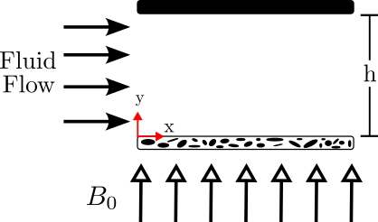
In this section, we describe the formulation of a MHD flow in a microchannel with an upper impenetrable wall and a lower penetrable porous wall. The boundary conditions of the flow are specified. The conditions refer to the no-slip condition at the upper wall, the slip velocity at the porous interface, and the Beavers-Joseph boundary condition (BJBC). For the closure of the problem, the BJBC is applied to the lower porous wall. The problem investigated here is the flow of an electrically conducting Newtonian fluid in a microchannel with an upper boundary impenetrable and a lower one consisting of a porous boundary. The fluid is undergoing a transverse and uniform magnetic field.
As the lower boundary is porous, we shall apply the semi-empirical boundary condition of Beavers and Joseph[5]. A schematic of the flow problem explored here can be seen in Figure 1. The small distance between the walls of the micro-channel is h, and B0 is the uniform and transverse external magnetic field applied to the flow, Miranda et al. [11].
In this work the induced magnetic field is assumed as being:

where Bx is the longitudinal component of the induced magnetic field, and B0 is the transversal component of the applied field.
Make the governing equation non-dimensional is an essential step in solving flow problems. We use this approach to reduce the level of complexity and the number of variables in the model. Typical scales of the flow problem explored here are present in Table 1.
Table 1. Typical flow properties and scales used to make the flow problem non-dimensional.
|
Property |
Typical scales |
|
Length |
h |
|
Pressure |
ηum/h |
|
Velocity |
um |
|
Electric field |
umB0 |
|
Magnetic Flux Density |
B0 |
Therefore, the non-dimensional quantities are given by:
where Bo is the applied magnetic induction and we take the one as a reference scale in the present formulation. Additionally, the pressure is denoted by p. The external electric field is E0. The velocity in the x-direction is vx, and the film velocity in the porous medium is um,. The classical Darcy's law describes the low Reynolds number flow in a porous medium. As a typical velocity scale, we use this velocity in porous medium facing the lower wall. First, however, we are going to use it to make the velocity non-dimensional. Relevant physical parameter in this flow is the Hartmann number which measures the relative importance between magnetic and viscous forces: Ha=B0h√(ke/η), where ke and η are the electrical conductivity and viscosity of the fluid, respectively [7]. Another non-dimensional parameter is the Magnetic Reynolds number (ratio between the diffusion time and the advection time of B): Rem=hum/νm, where νm is the magnetic diffusion coefficient [7]. Both parameters Hartmann and magnetic Reynolds number are based on the distance h between the walls as suggested in Miranda et al. and Sinzato and Cunha [11], [12].
2.1. Hydrodynamic Equations
For the purely hydrodynamic flow, the problem has the same configuration as Figure 1 except for the applied magnetic field B.
2.1.1. Governing Equations
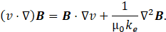
Considering a steady unidirectional flow (free of inertia) of an incompressible Newtonian fluid, the basic balance equations are [13]:
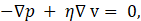
with ∇⋅v = 0.
Eq. 3 is a simplified version of the Navier-Stokes equations (NS) for pure viscous flow. We are considering steady-state conditions, with constant viscosity and no effects of body forces, as the net effect of the hydrostatic influence of gravity is included in the pressure term, as a modified pressure given by p=p'-ρg.x.
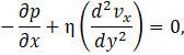
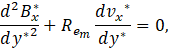
Under condition of a lubrication regime, Re (h/L) ≪ 1, the components x, y and z of the Eq. 3 are given respectively by:


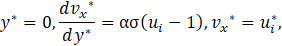
with the following associated boundary condition in the lower and upper wall respectively:
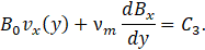
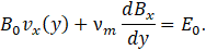
Note that, for calculating explicitly uih at the lower wall we must use the supplementary boundary condition:

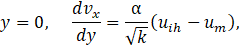
Here, uih is the slip velocity at the porous interface. The porosity is defined as being the ratio between the total volume of porous and the volume of the porous media. In addition, k is the permeability of the porous media which in more general case depends on the porosity. The quantity um is the average velocity in the porous medium (i.e. the flow rate over the area). Under the previous conditions, the creeping flow in a porous media is described by the classical Darcy law [13]:
Solving Eqs. 4-10 we found the solution for the flow case of a non-conducting fluid [5] :
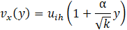
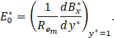
The solution in Eq. 11 gives the velocity component as a function of y and the pressure gradient. The interfacial velocity in the lower boundary is continuous and found when using the supplementary boundary condition given in Eq. 9. This results,
where σ=h/√k.
Now, when write Eq. 11 in terms of non-dimensional quantities we found:
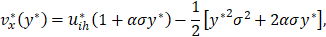
where the interface non-dimensional velocity ui is given by:
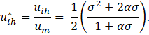
Note that ![]() is a crescent function of σ for a given α. However, as σ goes to zero, uih /um goes to zero as well, independent of α. In addition, for
is a crescent function of σ for a given α. However, as σ goes to zero, uih /um goes to zero as well, independent of α. In addition, for ![]() , and
, and ![]() , uih=um. In addition, for
, uih=um. In addition, for ![]() ,
, ![]() and if
and if ![]() ,
, ![]() . This simple analysis suggests how the shape of the velocity profile may change in the presence of a penetrable wall, depending on the permeability of the porous media facing the microchannel.
. This simple analysis suggests how the shape of the velocity profile may change in the presence of a penetrable wall, depending on the permeability of the porous media facing the microchannel.
2.2 Magnetohydrodynamic Equations
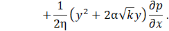
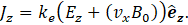
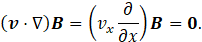
The current density is evaluated by the classical Ohm’s as follows [7].

where ke is the electric conductivity of the fluid and E denotes eletric field.
As the velocities components in y and z directions are both null and in the absence of magnetic field in z direction, Eq. 15 reduces to:
Now, from Faraday’s law for steady-state flow:
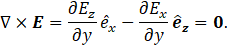
Eq. 17 leads to: Ez=E0 for any y. Consequently:
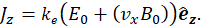
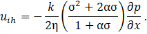
In addition, the current density can also be written in terms of the derivative of Bx. Using Ampere’s law [14]. We found:
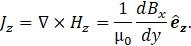
Now, combining Eq. 18 and Eq. 19, we can write the derivative of Bx with y in terms of E0, B0 and vx as follows:
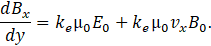
Using Eq. 18 and the magnetic induction given by Eq. 1, we found:

where fL denotes Lorentz Force.
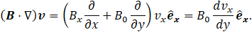
Now, substituting Eq. 21 into the Navier-Stokes equation in the presence of the MHD force, (i.e. Lorentz force per unit of volume) we obtain:

In terms of x, y, z, components Eq. 22 can be expressed in the following form:
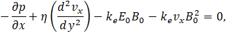
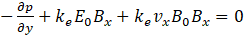

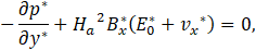
The closure formulation of the MHD flow examined requires the equation of magnetic inductions transport given by [7]:
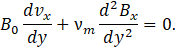
In Eq. 26, the νm=1/(μ0ke) is defined as the magnetic diffusion coefficient. Note that under condition of unidirectional flow the transport of the magnetic induction field by flow convection is null, that is:
On the other hand, the stretching of the magnetic induction by the flow can be calculated as follows:
Therefore, using the expressions given by Eq. 27 and Eq. 28, the transport of B reduces to:
Now, the system of the governing equations of the MHD flow with the associated boundary conditions can be written in terms of non-dimensional variables as follows:
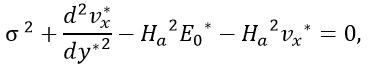


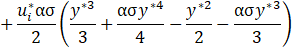
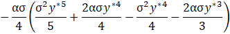
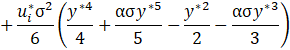
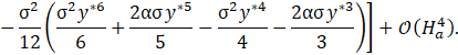
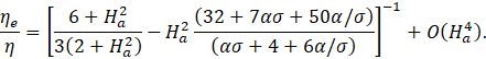
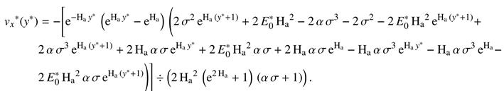
The exact solutions of the Eq. 30, Eq. 31, and Eq. 32 were obtained using the symbolic solve for ordinary differential equations - MATLAB software. In this way, the velocity field, the magnetic flux density, the pressure field, flow rate, and induced electric field are analytically determined and the associated exact expressions are presented in the Appendix of this work. However, these equations are not presented in this work, because they are too long and tedious even to be presented as an Appendix in the work. We shall make the huge expressions of the exact solutions available to the readers as a supplementary material. However, in substitution to the exact expressions, we provide an asymptotic solution sufficient to explore in detail the flow problem examined here. Although simpler, the asymptotic solutions give the same physical insights of the flow for Ha<1.
2.3. Method of solution
In this section we shall describe the method of solution in order to solve the flow problem of the MHD microchannel flow. Say, velocity field, flow rate, pressure field, magnetic induction and an effective viscosity of the flow. The expressions presented here will be used in section (3) where a regular asymptotic solution is developed to find the leading order contribution to the flow solution O(Ha2 ).
2.3.1. Velocity Field and Flow Rate
The flow velocity can be calculated directly by solving the second order differential Eq. 30 with the boundary conditions given by Eqs. 33-36. Note that the boundary conditions will be used in this solution, similarly to the pure hydrodynamic case (i.e. Ha=0). The velocity field must be integrated to find the non-dimensional flow rate in the channel, namely
2.3.2. Magnetic Flux Density
The magnetic induction may be determined by rearranging two integrations concerning y^* in Eq. 32:
Now to find the integration constants C1 and C2, two magnetic boundary conditions of the problem must be used. These conditions are Bx*(y*=0)=Bx* (y*=1)=0. Additionally, substituting the result of the velocity field in Eq. 37 and after integrating and making some algebraic manipulations, we found the non-dimensional flow rate.
2.3.3. Pressure Field
The pressure gradient is constant along the axis, as seen throughout this work:

After integrating Eq. 39, it results:

Here f(y*) as a direct consequence of Eq. 40, we have:
Now, substituting the pressure gradient given in Eq. 31 into Eq. 41, we have:
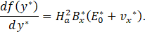
The pressure field is found by solving Eq. 42 for f(y*) and substituting it into Eq. 40.
2.3.4. Electric field
The electric field can be determined by first integrating Eq. 29 that results:
Note that C3 is just an integration constant. Substituting Eq. 20 into Eq. 43, it results

Hence, applying the boundary condition y=h⇒vx=0, we have that E0=C3. Therefore, Eq. 43 takes the form:
.
Now, writing Eq. 45 in terms of non-dimensional quantities and using the wall no-slip boundary condition, we can calculate one expression for the non-dimensional electrical field as follows:
3. A Regular Asymptotic Solution
As mentioned before, the exact solution for Eq. 30, when solved by using the symbolic solve for ordinary differential equations - MATLAB software results in a complicated expression where the contribution of the magnetic field is not straightforward to be separated from the leading order solution O(1) (see Appendix). Therefore, the exact solutions are not suitable to explore the flow phenomenon in the presence of MHD effects from a physical point of view. In contrast, a regular asymptotic solution of the flow O(Ha2) seems to be useful for splitting the solution of the problem into two main contributions: a purely hydrodynamic term O(1), that is the leading order contribution and a correction O(Ha2) due to magnetic effects. The asymptotic solution although simpler and an approximation of the exact solution provide the same physical insights of the channel pressure driven flow for Ha<1. Consequently, the interpretation of the physical mechanisms involved in the flow can be better understood and discussed.
Using a regular perturbations method described in [15], [16], the velocity field can be expressed as:

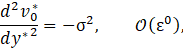
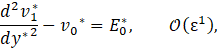
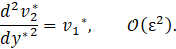
where, in the flow problem examined here, the small parameter ε=Ha2. Then, substituting Eq. 47 into Eq. 30 and after a few algebraic manipulations, we find the following system of ordinary differential equations at different order of ε:
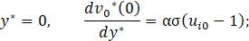
Since the solution of the velocity field is given by a regular asymptotic expansion, then the velocity at the interface with the porous medium can be also represented in terms of a regular expansion in orders of ε:

So, the boundary conditions are:
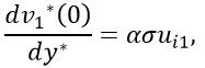

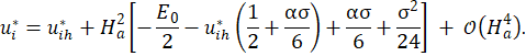
Now, Eq. 48 just represents the purely hydrodynamic contribution since - σ2 is defined as the pressure gradient as it has been expressed in Eq. 39. On the other hand, Eq. 49 and Eq. 50 correspond to the MHD contribution. Therefore, we can obtain the velocity with a truncation error O(Ha2) as following:

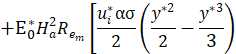
where v0* is the leading order of the solution and given by Eq. 13 and v1* is given by:

Now, if Ha<1, it means that ε ≪ 1 (small parameter), so the method gives a highly accurate solution in this regime. As Ha increases, the asymptotic solution diverges from the exact solution of the Eq. 30, as we can verify in Figure 5. This means that the terms of higher order cannot be neglected in this regime since the Hartmann number is no longer small, Miranda et al. [11].
Solving the third boundary condition determines the velocity at the porous medium interface. Once solved using the perturbation method, the interface velocity will also be expressed as an asymptotic expansion in terms of the Hartmann number, according to equation X. Again, it is possible to detect in the solution the hydrodynamic contribution and the MHD contribution, which scale with orders of the Hartmann number. If the Hartmann number is very small, approaching zero, the velocity at the porous medium interface recovers the interface velocity obtained in the purely hydrodynamic problem.
Now, using the asymptotic expansion for the velocity field in Eq. 55, we determine the asymptotic solution for the magnetic induction field in the x direction solving Eq. 38 as after some algebraic manipulations we have


Here the non-dimensional electric field E0* can be determined through the Eq. 46. Therefore

Using the Eq. 37, we can determine the flow rate, splitting the solution in a purely hydrodynamic contribution and a MHD correction O(Ha2 ), we obtain
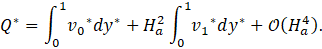
Solving Eq. 60 results in

Finally, we also propose an asymptotic solution for the pressure distribution in the microchannel solving Eq. 39 for the non-dimensional pressure gradient in y^* direction. After substituting the solution into Eq. 40, it results:
4. Effective Viscosity
Another important quantity of the flow is the effective viscosity, which measures the increase in the fluid dissipation produced by MHD effects. The effective viscosity here is defined as the one which an electrically conducting fluid should have to behave like a non-conducting Newtonian fluid subject to the same pressure gradient. Therefore, the effective viscosity will naturally depend on Ha. In the context of the blood flow, this quantity is called intrinsic or equivalent viscosity of the flow that is frequently used in practical applications of hemorheology [17], [18]. Due to the deceleration in the flow produced by MHD as a transversal magnetic field is applied, we can associate this extra dissipation with an increase in the fluid viscosity.
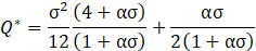
An expression for the effective viscosity can be obtained when comparing the flow rate under MHD effect given in Eq. 61 with the Poiseuille law of the channel flow given for a non-conducting Newtonian fluid (Ha=0) given by:
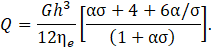
Therefore, comparing Eq. 61 and Eq. 63, we find the following expression for ηe/η:
5. Results and Discussion
In this section we present some results for the velocity and magnetic induction profiles in the microchannel unidirectional flow examined here. In addition, the effective viscosity, non-dimensional maximum velocity, the interface velocity facing the porous media and the flow rate as a function of the Hartmann number are also presented and discussed here. As the Hartmann number increases, the effects of the magnetic forces dominate the viscous forces, and the flow decelerates. This indicates that the MHD effect introduces an extra dissipation in the flow, which corroborates with the observed increase in the effective viscosity as Ha increases as shown in the plot of Figure 2. Note that the non-dimensional effective viscosity can be calculated by our asymptotic solution given in Eq. 64. The effect of the effective viscosity in the present context represents the dissipation in an equivalent Newtonian fluid undergoing the same pressure gradient, but with a viscosity higher than the viscosity of the electrically conducting fluid in the absence of magnetic (i.e. Ha=0). Of course, as Ha goes to zero the non-dimensional effective viscosity tends to 1 as can be seen in Figure 2.
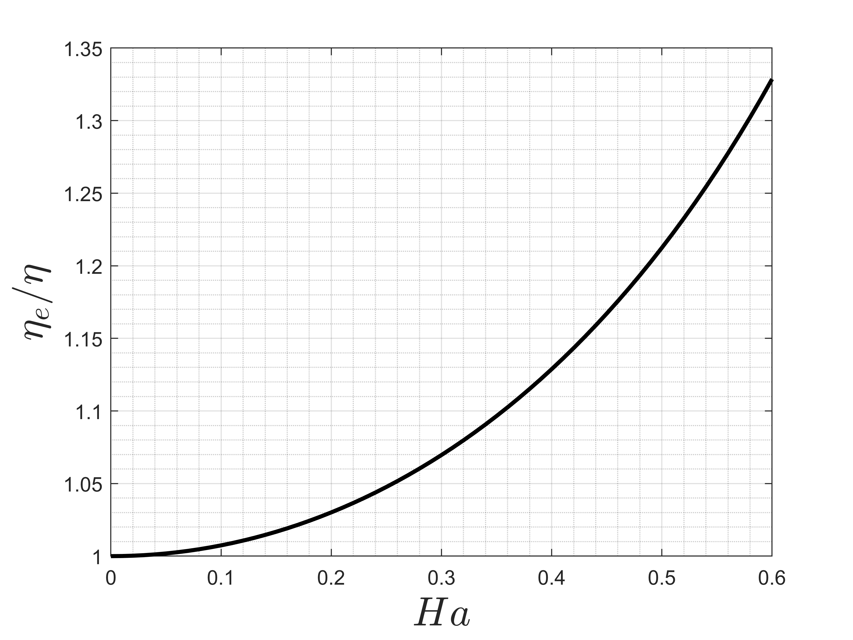
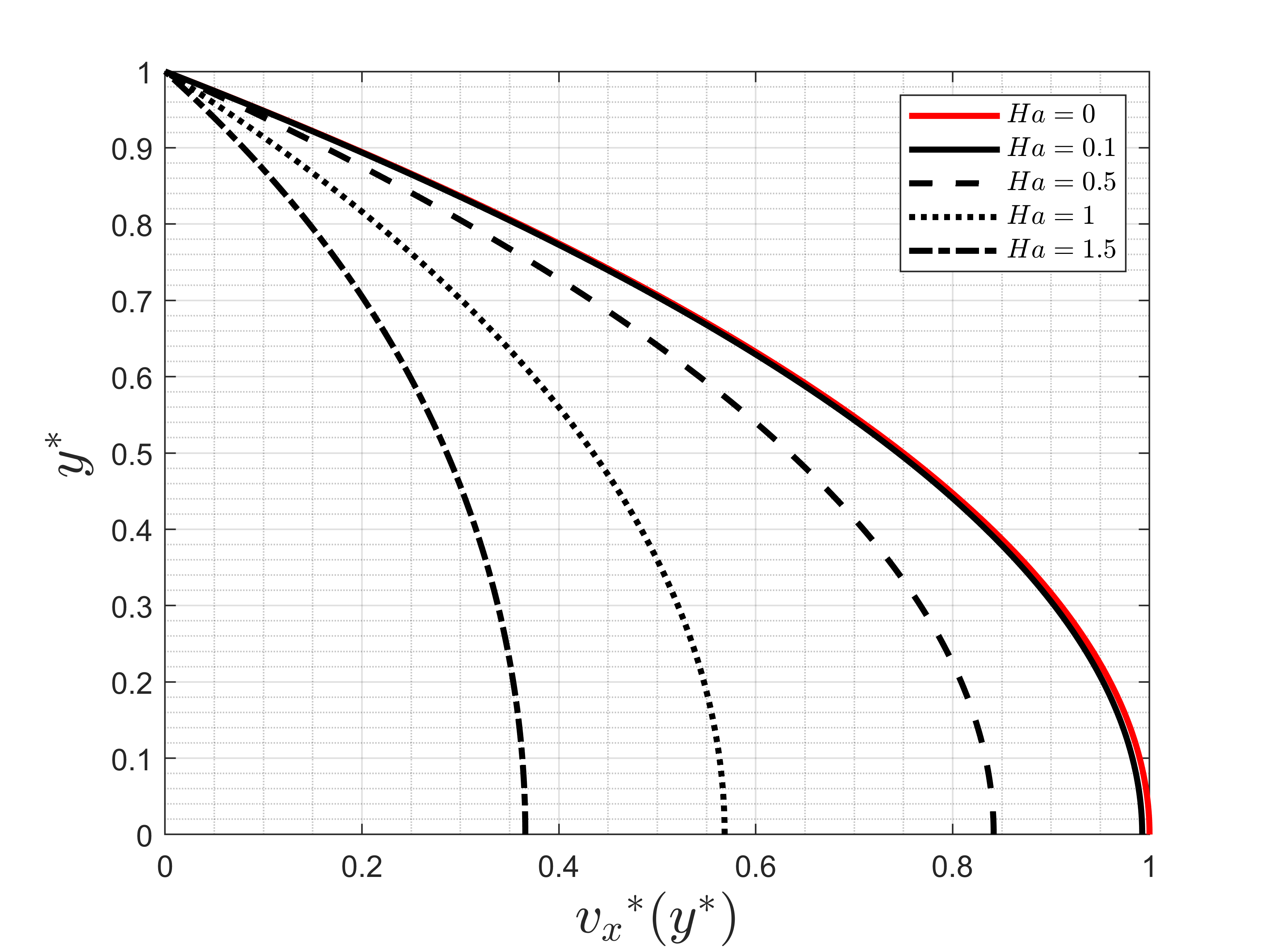
Figure 3 shows a typical velocity profiles of the non-dimensional x-component of the velocity as a function of the no-dimensional coordinate y*. We can clearly see that the velocity profile becomes flatter as Ha increases in the flow, moving away from the standard parabolic profile as Ha=0. We still emphasize that when the Hartmann number approaches zero, the MHD flow goes to the limit of the solution of a non-conducting Newtonian fluid experiencing the same pressure gradient. The convergence of the profiles in the limit of Ha → 0 is clearly seen as comparing the velocity profile for Ha=0 with the one for Ha=0.1. Additionally, it is interesting to observe that the tendency of a velocity profile to be more uniform rather than parabolic as a consequence of the flow dissipation by MHD effects is similar to the behavior of the velocity profiles in the pepe flows of shear thinning fluids with shear rate dependent viscosity.
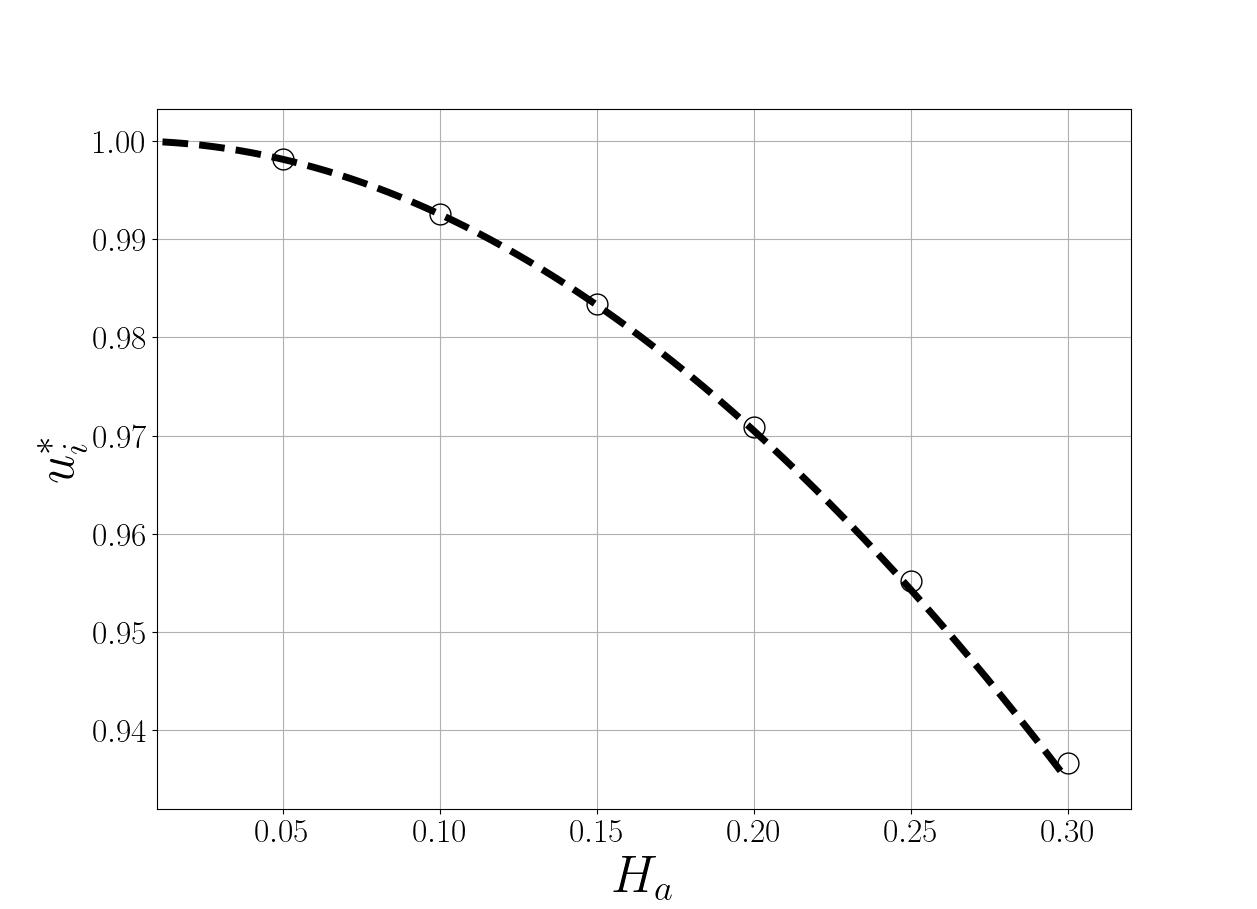
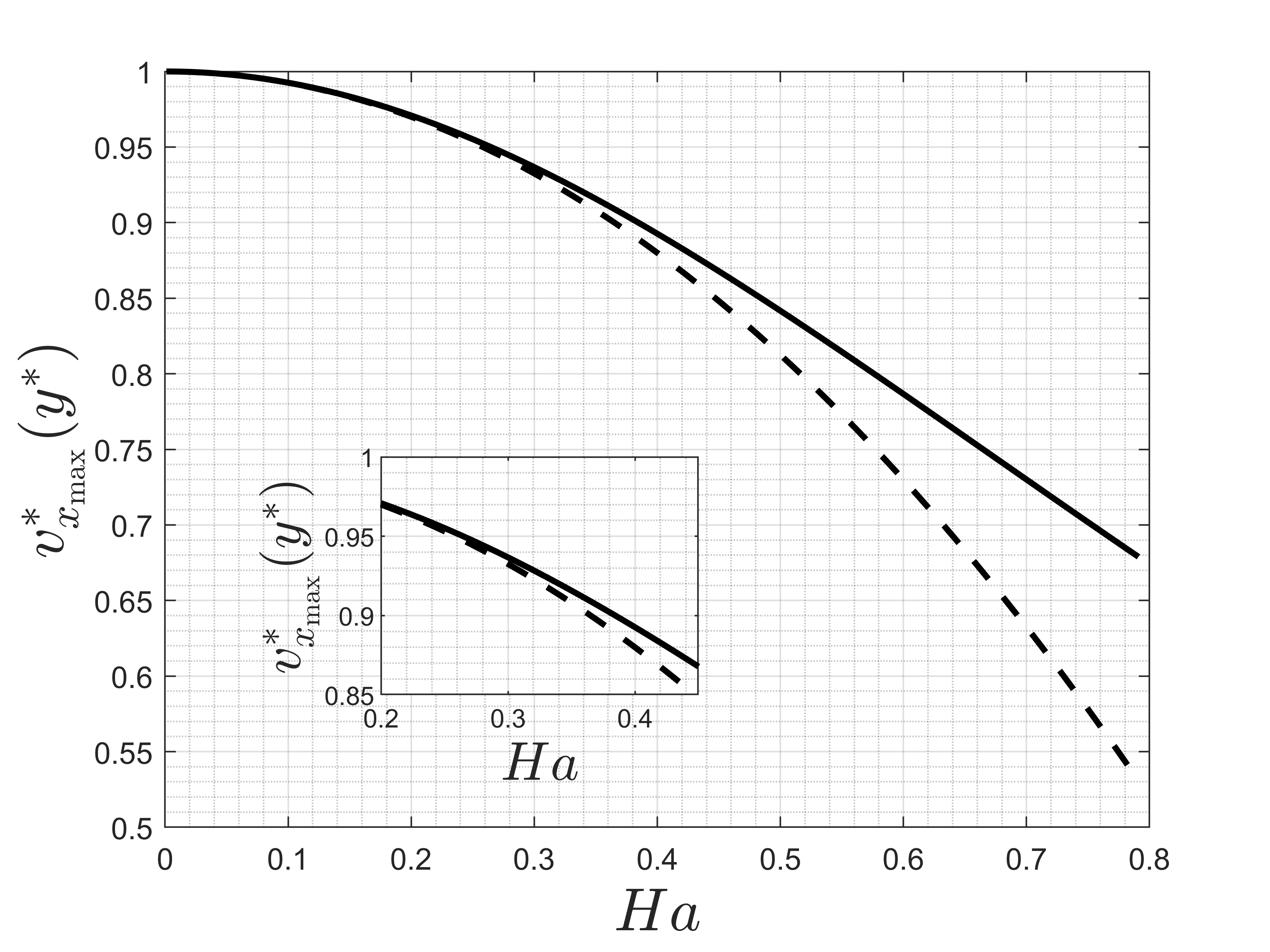
Figures 4, 5 present the behavior of the non-dimensional velocity at the porous medium interface (lower channel wall) and the maximum velocity, respectively, as Ha increases. As previously observed in Figure 3, the magnetic effects counteract the hydrodynamic effects, generating a "braking" effect on the flow. Therefore, it is natural that the interface velocity decreases with the increase of the Hartmann number, which means the growth of the flow dissipation by magnetic effects. It is seen that for a zero Hartmann number, the non-dimensional velocity at the interface corresponds to the condition of the purely hydrodynamic case, which equals 1 for the conditions of σ=√2 and σ=1/2. Under this condition, the interface velocity is the same as the mean velocity of the porous medium. The points in the plot represent the numerical values given by the exact solution expressions. As we can see the asymptotic solution for this quantity is in a perfect agreement with the exact solution for Hartmann numbers less than one. By analyzing the relative error between the exact and asymptotic solutions, it is found that for Ha=0.1, the error is 2.5×10⁻³%, and for Ha=0.3, it is 2.0×10⁻¹%. In other words, the difference between the two solutions is truly minimal, and in this Hartmann regime, the solution obtained by the perturbation method is a perfect alternative.
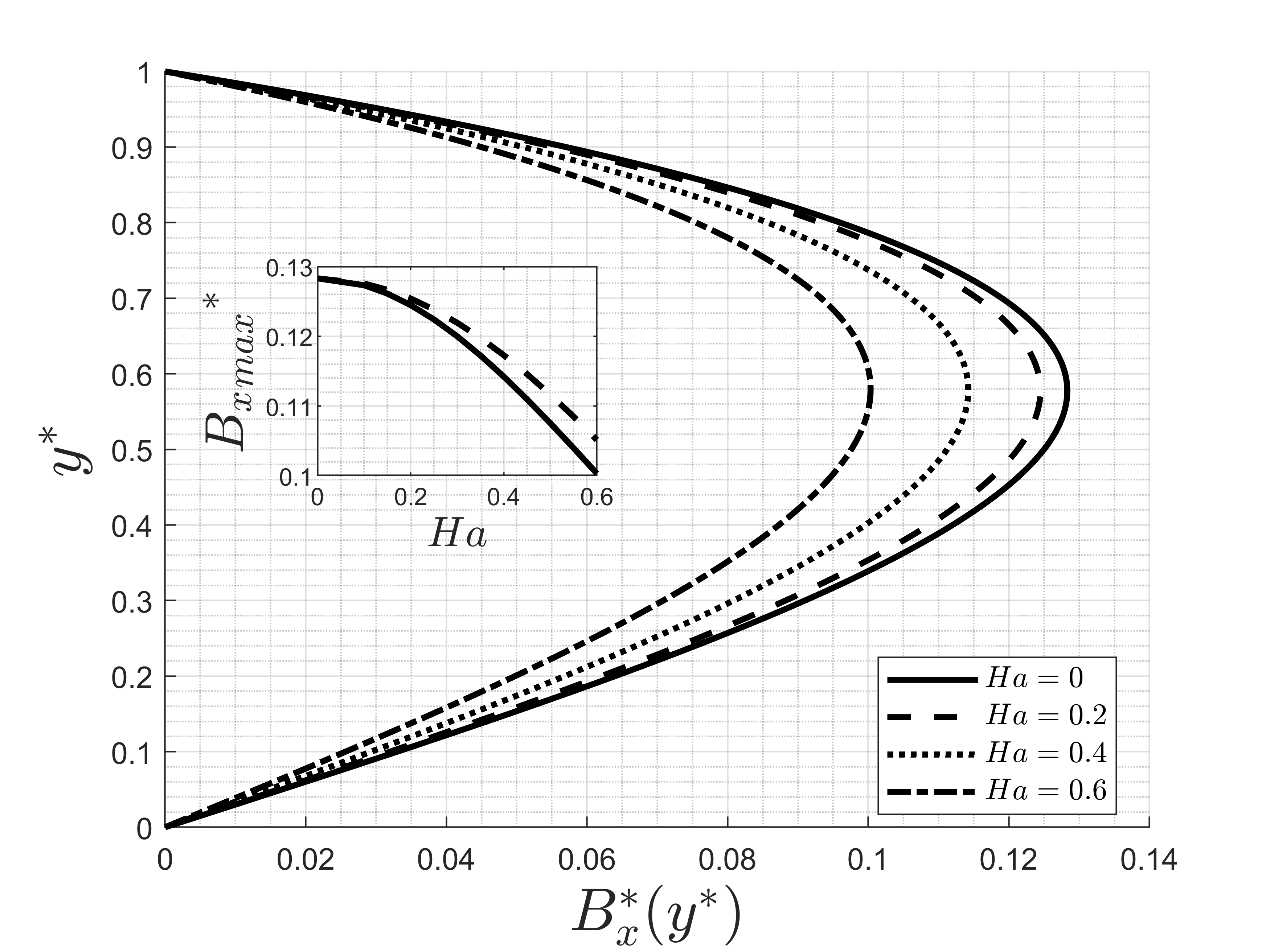
Additionally, Figure 6 shows the coupling between the induced magnetic flux density and the flow velocity. As Hartmann increases, the effects of the Lorentz force slow down the flow, making the maximum values of the induced magnetic flux absolute values smaller as can be seen by the inset of the Figure 6.
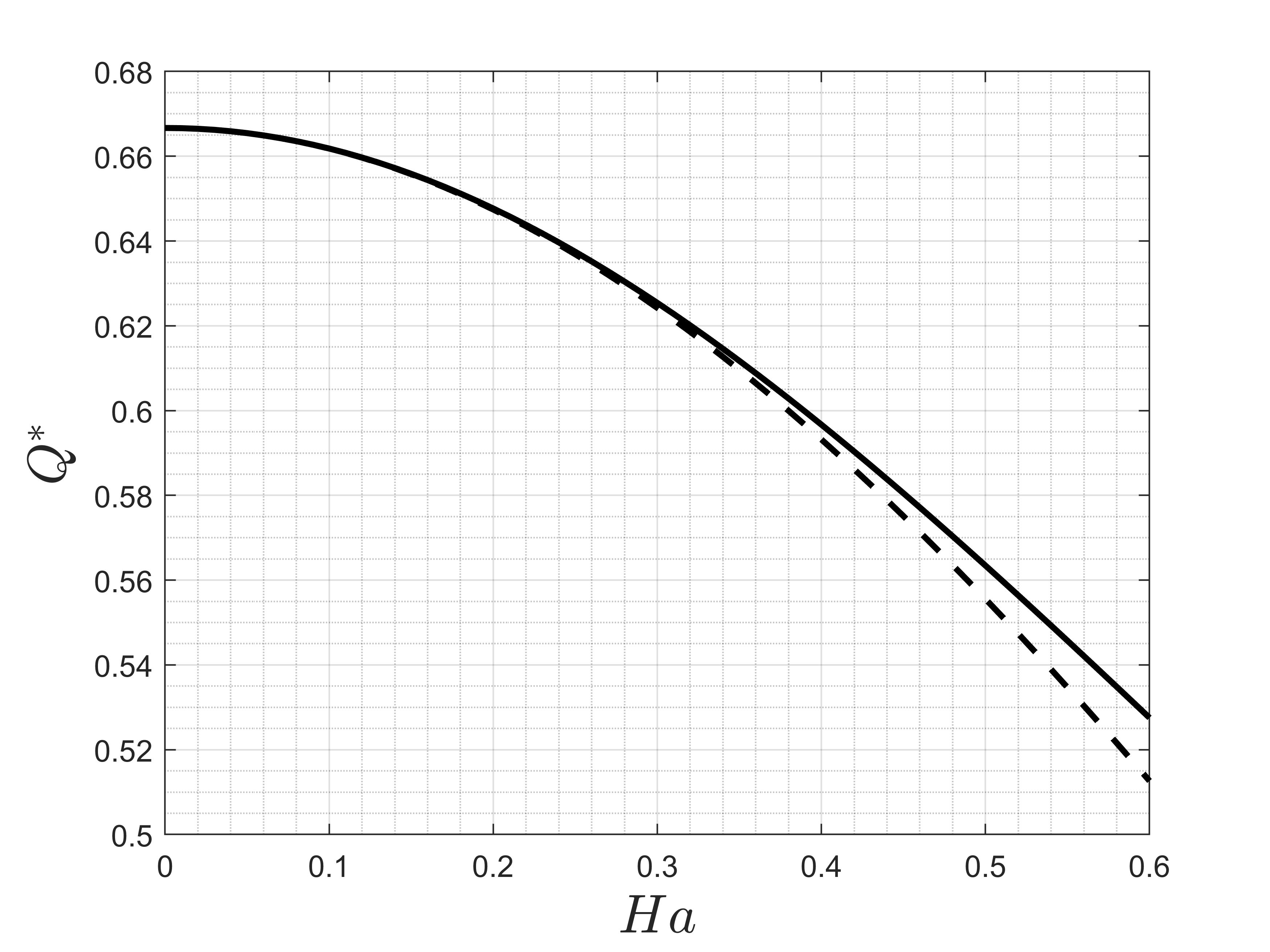
Figure 7 presents a plot of the flow rate as a function of the Hartmann number. If the Lorentz force is strong, the flow rate in the channel substantially decreases as a direct consequence of an increase of the flow dissipation rate by the magnetic field. The flow rate clearly decays with the increase of Hartmann, as pointed out by Figure 7. As a complementary result Figures 8 and 9 show that the channel flow can be accelerate at the interface wall with the porous media by increasing the permeability parameter σ. Figure 8 clearly shows perceptible variations in the velocity profile shape when the permeability of the porous media or the channel gap are changed. Actually, an increase in the parameter σ means to decrease the permeability of the porous media. In this case, the mean velocity in the porous media is decreased and the ratio, uih/um increases with σ linearly for both Ha as depicted in Figure 9. For Ha=0.3 the interfacial velocity in the lower wall is just slightly lower than the same for Ha=0 and the ratio uih/um is pretty close to unit for σ=√2. Additionally, it is interesting to note that the average velocity of a liquid in porous media flows could be controlled by monitoring both the electrical and, or the magnetic field without changing the porous media characteristic that would be certainly unusual and difficult from a practical point of view.
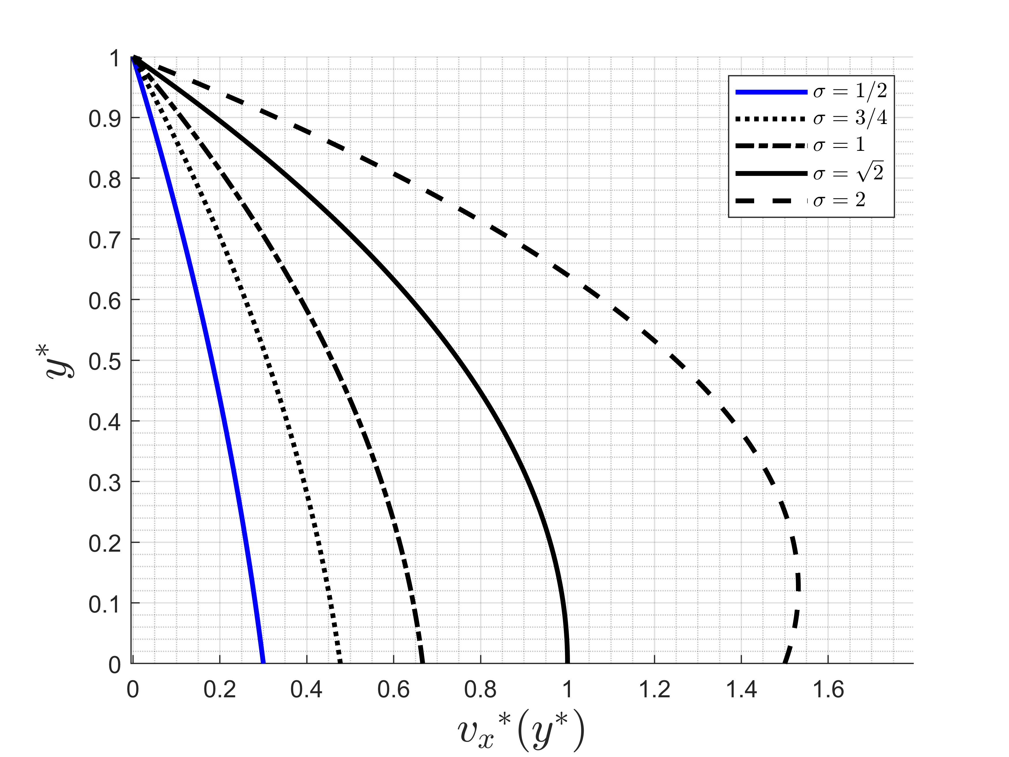
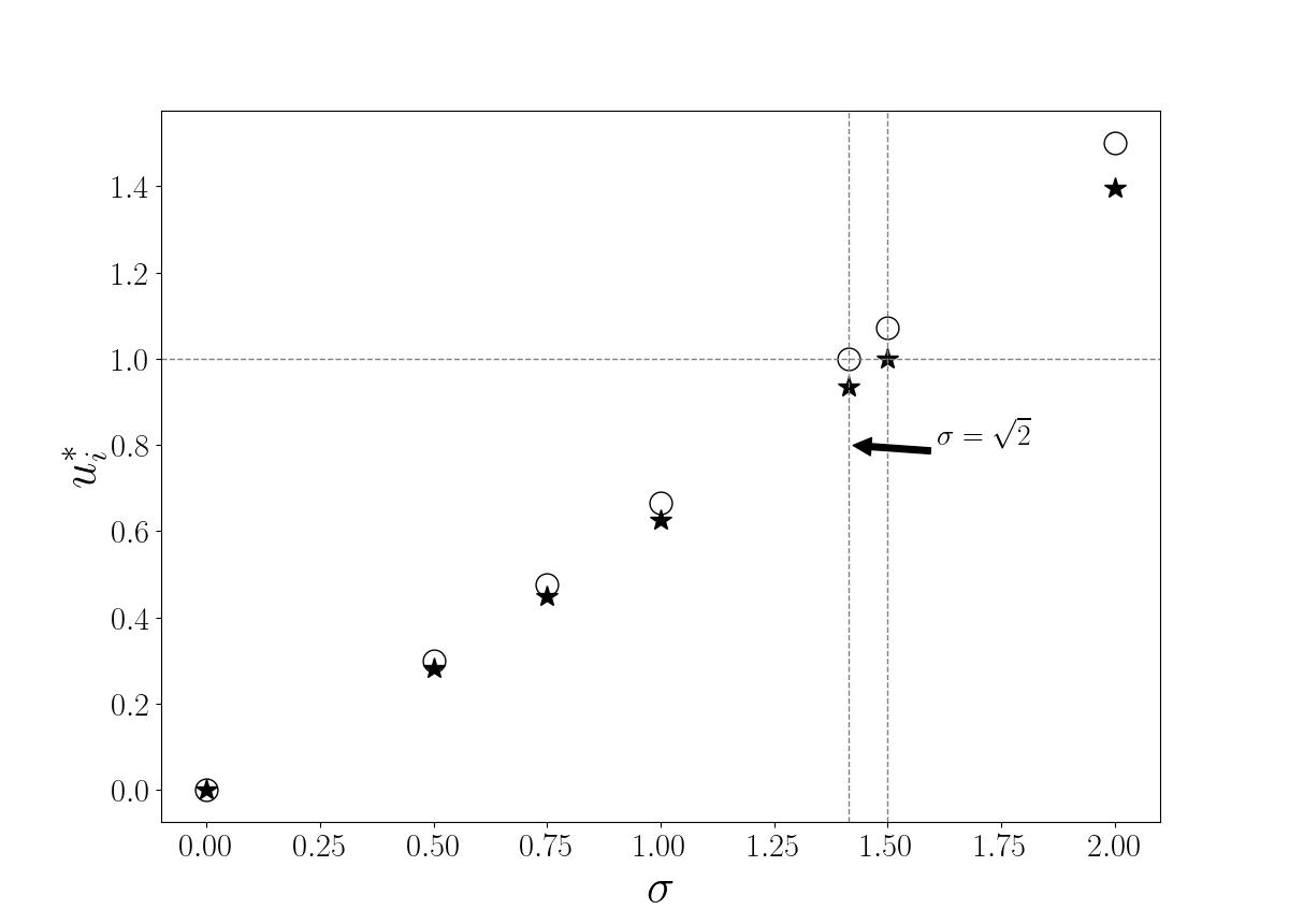
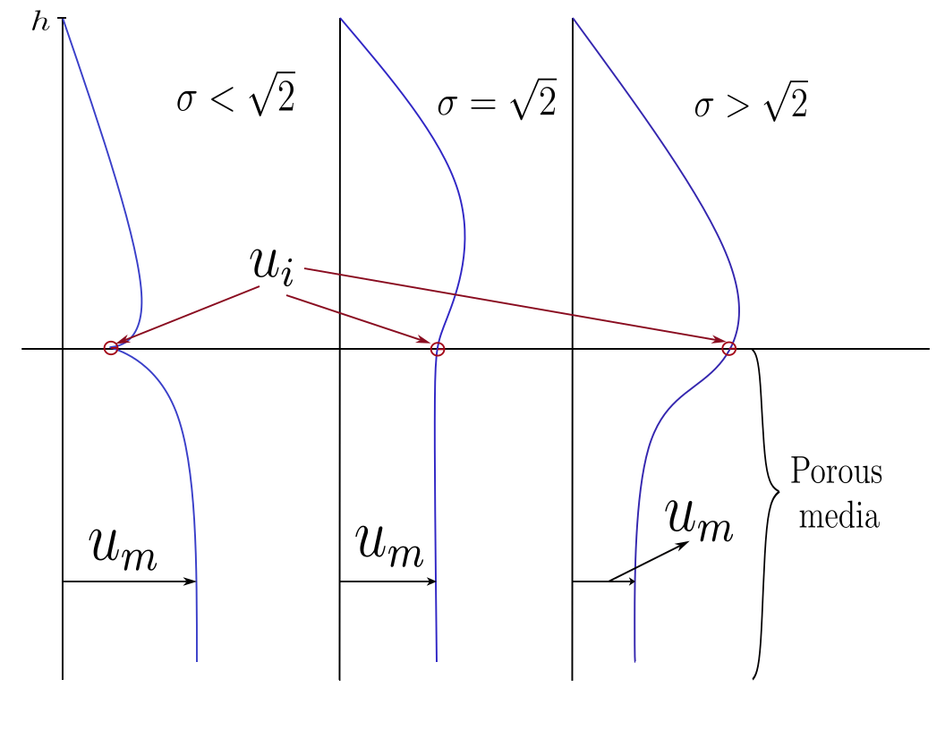
The sketch of the full velocity profile, including the porous media facing the channel lower wall is shown in Figure 10. As already seen in Figure 9, For the purely hydrodynamic flow corresponding to Ha = 0, when σ<√2 means higher permeability of the porous medium. This condition results in the porous media mean velocity being greater than the interfacial velocity. Otherwise, σ>√2 corresponds to smaller values of permeability, and the mean velocity in the porous medium is smaller than the interfacial velocity. This range of the mean velocity in a porous media by changing the permeabilities can be also defined by controlling the intensity of electric and magnetic fields as using an electrically conducting fluid. Several applications require very low percolation velocities in a porous media such as in soil mechanics in agricultural applications. The dependence of the non-dimensional interfacial velocity on the σ parameter is plotted in Figure 10. We can see that in the presence of MHD effect on the flow, the value at which the interfacial velocity is equal of the porous media velocity is slightly different of √2 (i.e. σ≈1.5). The attenuation effect on the flow caused by the transverse magnetic field could be also interpreted as an equivalent increase in the permeability of the porous medium, as if it were possible to change the permeability of the porous medium (which is a more structural aspect) by merely increasing the intensity of the external magnetic field. This effect seems to be a relevant MHD application in the context of porous media explored here.
Essentially, the boundary condition used for the channel lower wall interfacing a porous medium makes the flow to resemble the one which occurs in the tiny pores of natural reservoirs during oil extraction by a pressure-driven flow. This interesting finding in this work may provide insight into developing numerical simulations to explore nonlinear regimes of the flow for different intensities of the magnetic field, the presence of inertia, and different conditions of the porous media facing the lower wall as porosity and permeability. We plan in future work to explore the effect of drag reduction by magnetic pumping and the equivalent effect of decreasing permeability of a porous medium using magnetic deceleration.
6. Conclusion
In this work, the results have shown how magnetohydrodynamic force can modify the velocity field, the pressure field, the induced magnetic field and dissipation in a microchannel flow with a penetrable wall facing a porous media undergoing different conditions of permeability and intensity of a transversal magnetic field. Indeed, the MHD effect produces a deceleration in the flow, increasing the rate of dissipation in the fluid. This increase in dissipation may be characterized by an effective viscosity, which depends on the Hartmann number. In addition, we can produce an effect of magnetic pumping flow by controlling both the electrical and the magnetic fields on the conducting fluid.
The asymptotic solutions of the flow problem examined here were important to split the solution in two parts: a purely hydrodynamic contribution and a leading order contribution in terms of Ha2. In particular, the asymptotic solutions, although simpler, have provided the same physical insights for Ha<1 and are much easier to be manipulated. Additionally, the slip condition in the porous wall modifies the flow dynamics since the velocity is not zero in the lower penetrable wall as occurs in the upper wall. This effect can be also changed by controlling the porosity and the permeability of the porous media facing the channel in the lower wall. We found that the shape of the velocity profile in the microchannel can be strongly influenced by the permeability of the porous interfacing the lower wall. For the permeability parameter σ which corresponds to the reciprocal of the non-dimensional permeability root square equal to √2 and porosity fixed and to ½ the interface velocity in the channel wall is exactly the same the average velocity in the porous media. On the other hand, if the same parameter is less than √2 the interfacial velocity is always less than the porous media velocity. Otherwise, the interfacial velocity is greater than the porous media mean velocity. Therefore, the application of a transverse magnetic field in the flow of an electrically conducting fluid in tiny pores can produce an effective effect like the flow deceleration which occurs as the porous media permeability is decreased. It seems to be possible to produce such an effect by just monitoring the magnetic field instead of changing the complex microstructure of the porous medium. On the other hand, for flow applications where the magnetic pumping effect is necessary, control of the intensity of the electric field is always required.
References
[1] L. Bühler, "Instabilities in quasi-two-dimensional magnetohydrodynamic flows," J Fluid Mech, vol. 326, pp. 125-150, Nov. 1996, doi: 10.1017/S0022112096008269.
View Article
[2] H. H. Bau, J. Zhong, and M. Yi, "A minute magneto hydro dynamic (MHD) mixer," Sens Actuators B Chem, vol. 79, no. 2-3, pp. 207-215, Oct. 2001, doi: 10.1016/S0925-4005(01)00851-6.
View Article
[3] R. A. Alpher, "Heat transfer in magnetohydrodynamic flow between parallel plates," Int J Heat Mass Transf, vol. 3, no. 2, pp. 108-112, Sep. 1961, doi: 10.1016/0017-9310(61)90073-4.
View Article
[4] V. A. Bityurin, A. N. Bocharov, and N. A. Popov, "Magnetohydrodynamic deceleration in the Earth's atmosphere," J Phys D Appl Phys, vol. 52, no. 35, p. 354001, Jul. 2019, doi: 10.1088/1361-6463/AB2181.
View Article
[5] G. S. Beavers and D. D. Joseph, "Boundary conditions at a naturally permeable wall," J Fluid Mech, vol. 30, no. 1, pp. 197-207, Oct. 1967, doi: 10.1017/S0022112067001375.
View Article
[6] F. R. Cunha, "Nonlinear effects in Porous Media flow with Permeable interface," Journal of the Brazilian Society of Mechanical Science and Engineering, vol. 2, pp. 107-135, 1991.
[7] P. A. Davidson, "Introduction to Magnetohydrodynamics," Introduction to Magnetohydrodynamics, Dec. 2016, doi: 10.1017/9781316672853.
View Article
[8] P. H. Roberts, "An Introduction to Magnetohydrodynamics."
[9] S. Ganesh and R. Delhi Babu, "Steady MHD flow between two parallel porous plates with an angular velocity," International Journal of Ambient Energy, vol. 42, no. 13, pp. 1529-1537, 2021, doi: 10.1080/01430750.2019.1611647.
View Article
[10] P. Chandrasekar, S. Ganesh, A. M. Ismail, and V. W. J. Anand, "Magnetohydrodynamic flow of viscous fluid between two parallel porous plates with bottom injection and top suction subjected to an inclined magnetic field," AIP Conf Proc, vol. 2112, no. 1, Jun. 2019, doi: 10.1063/1.5112329/1024198.
View Article
[11] É. M. Miranda, M. F. de S. A. Filho, and F. R. Cunha, "Bounded Pressure-Driven Flow of an Incompressible Electrically Conducting Fluid: Porous Medium and Lubrication Applications," Jun. 2024. doi: 10.11159/ffhmt24.078.
View Article
[12] Y. Z. Sinzato and F. R. Cunha, "Stability analysis of an interface between immiscible liquids in Hele-Shaw flow in the presence of a magnetic field," Appl Math Model, vol. 75, pp. 572-588, Nov. 2019, doi: 10.1016/j.apm.2019.05.049.
View Article
[13] G. K. Batchelor, An Introduction to Fluid Dynamics. Cambridge University Press, 1967.
[14] D. J. Griffiths, Introduction to Electrodynamics, 4th ed. Cambridge University Press, 2017.
View Article
[15] E. J. Hinch, "Perturbation Methods," Perturbation Methods, Oct. 1991, doi: 10.1017/CBO9781139172189.
View Article
[16] J. Logan, Applied mathematics. John Wiley & Sons, 2013.
[17] A. S. Popel and P. C. Johnson, "Microcirculation and hemorheology," 2005. doi: 10.1146/annurev.fluid.37.042604.133933.
View Article
[18] G. Roure and F. R. Cunha, "Modeling of unidirectional blood flow in microvessels with effects of shear-induced dispersion and particle migration," Appl Math Mech, vol. 43, no. 10, pp. 1585-1600, 2022.
View Article
Appendix
This section presents the equations for the exact solutions developed in this work by using the symbolic solve for ordinary differential equations - MATLAB software.
Velocity Field
Slip Velocity

Flow Rate
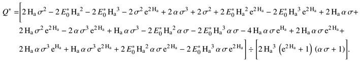
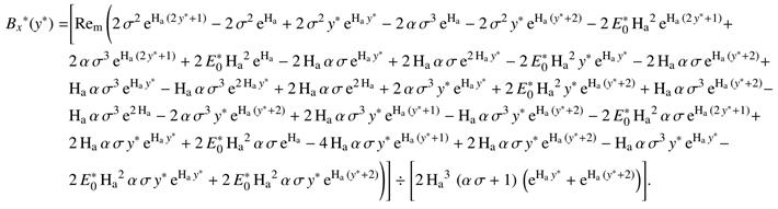
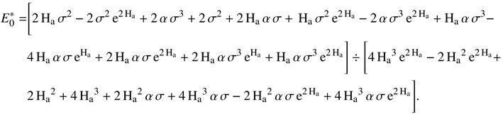
Magnetic Flux Density
Electric Field
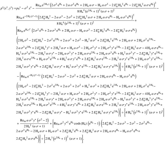
Pressure Field
[1] L. Bühler, "Instabilities in quasi-two-dimensional magnetohydrodynamic flows," J Fluid Mech, vol. 326, pp. 125-150, Nov. 1996, doi: 10.1017/S0022112096008269. View Article
[2] H. H. Bau, J. Zhong, and M. Yi, "A minute magneto hydro dynamic (MHD) mixer," Sens Actuators B Chem, vol. 79, no. 2-3, pp. 207-215, Oct. 2001, doi: 10.1016/S0925-4005(01)00851-6. View Article
[3] R. A. Alpher, "Heat transfer in magnetohydrodynamic flow between parallel plates," Int J Heat Mass Transf, vol. 3, no. 2, pp. 108-112, Sep. 1961, doi: 10.1016/0017-9310(61)90073-4. View Article
[4] V. A. Bityurin, A. N. Bocharov, and N. A. Popov, "Magnetohydrodynamic deceleration in the Earth's atmosphere," J Phys D Appl Phys, vol. 52, no. 35, p. 354001, Jul. 2019, doi: 10.1088/1361-6463/AB2181. View Article
[5] G. S. Beavers and D. D. Joseph, "Boundary conditions at a naturally permeable wall," J Fluid Mech, vol. 30, no. 1, pp. 197-207, Oct. 1967, doi: 10.1017/S0022112067001375. View Article
[6] F. R. Cunha, "Nonlinear effects in Porous Media flow with Permeable interface," Journal of the Brazilian Society of Mechanical Science and Engineering, vol. 2, pp. 107-135, 1991.
[7] P. A. Davidson, "Introduction to Magnetohydrodynamics," Introduction to Magnetohydrodynamics, Dec. 2016, doi: 10.1017/9781316672853. View Article
[8] P. H. Roberts, "An Introduction to Magnetohydrodynamics."
[9] S. Ganesh and R. Delhi Babu, "Steady MHD flow between two parallel porous plates with an angular velocity," International Journal of Ambient Energy, vol. 42, no. 13, pp. 1529-1537, 2021, doi: 10.1080/01430750.2019.1611647. View Article
[10] P. Chandrasekar, S. Ganesh, A. M. Ismail, and V. W. J. Anand, "Magnetohydrodynamic flow of viscous fluid between two parallel porous plates with bottom injection and top suction subjected to an inclined magnetic field," AIP Conf Proc, vol. 2112, no. 1, Jun. 2019, doi: 10.1063/1.5112329/1024198. View Article
[11] É. M. Miranda, M. F. de S. A. Filho, and F. R. Cunha, "Bounded Pressure-Driven Flow of an Incompressible Electrically Conducting Fluid: Porous Medium and Lubrication Applications," Jun. 2024. doi: 10.11159/ffhmt24.078. View Article
[12] Y. Z. Sinzato and F. R. Cunha, "Stability analysis of an interface between immiscible liquids in Hele-Shaw flow in the presence of a magnetic field," Appl Math Model, vol. 75, pp. 572-588, Nov. 2019, doi: 10.1016/j.apm.2019.05.049. View Article
[13] G. K. Batchelor, An Introduction to Fluid Dynamics. Cambridge University Press, 1967.
[14] D. J. Griffiths, Introduction to Electrodynamics, 4th ed. Cambridge University Press, 2017. View Article
[15] E. J. Hinch, "Perturbation Methods," Perturbation Methods, Oct. 1991, doi: 10.1017/CBO9781139172189. View Article
[16] J. Logan, Applied mathematics. John Wiley & Sons, 2013.
[17] A. S. Popel and P. C. Johnson, "Microcirculation and hemorheology," 2005. doi: 10.1146/annurev.fluid.37.042604.133933. View Article
[18] G. Roure and F. R. Cunha, "Modeling of unidirectional blood flow in microvessels with effects of shear-induced dispersion and particle migration," Appl Math Mech, vol. 43, no. 10, pp. 1585-1600, 2022. View Article
Appendix
This section presents the equations for the exact solutions developed in this work by using the symbolic solve for ordinary differential equations - MATLAB software.
Velocity Field
Slip Velocity
Flow Rate
Magnetic Flux Density
Electric Field
Pressure Field