Journal of Fluid Flow, Heat and Mass Transfer (JFFHMT)

ISSN: 2368-6111

Dynamic Characterization of Parametric Structures and Perturbation Analysis of Blood Flow in the Cranial Arteries

D. Otoo¹, K. Mensah¹, K. A. Adu-Poku², D. Gyamfi¹, B. A. Danquaah¹, H. Adusei³

¹University of Energy and Natural Resources, Department of Mathematics and Statistics
Box 214, Sunyani, 00233
²University of Energy and Natural Resources, Department of Mechanical and Manufacturing Engineering Box 214, Sunyani, 00233
³ Valley View University, Department of Science and Mathematics Education
dominic.otoo@uenr.edu.gh; kmensah33@st.knust.edu.gh; daniel.gyamfi@uenr.edu.gh; baaba.ghansah@uenr.edu.gh, hawa.adusei@yahoo.com

Abstract - Stroke is considered the second leading cause of death globally. The primary risk factor for stroke-related diseases is high blood pressure, which occurs as a result of insufficient blood transport to the brain due to blockages or ruptures in the blood vessels. This study presents the explicit finite-difference method through discretization of the solution domain of the 1-D Navier-Stokes equations capable of predicting pressure and flow profiles by characterizing key parameters of pressure variations inherent in the human cranial arteries. Interestingly, the results obtained shows that, the part of the wave with higher pressure travels faster to the periphery than the part with lower pressure. The increase in diastolic and a null decrease in systolic pressure as seen in our simulations is as a result of a slower heart rate, since the heart is taking longer time to complete a beat. Our findings shows that a decrease in the radius of the cranial artery from (0.29-0.275)cm will result in the increase in pressure within the range (115mmHg-145mmHg).

Keywords: Cardiovascular diseases, Systolic and diastolic pressures, 1-D Navier-Stokes equations, Explicit finite difference

© Copyright 2024 Authors - This is an Open Access article published under the Creative Commons Attribution License terms Creative Commons Attribution License terms. Unrestricted use, distribution, and reproduction in any medium are permitted, Pr ovided the original work is Pr operly cited.

Date Received: 2024-06-06
Date Revised: 2024-06-21
Date Accepted: 2024-07-24
Date Published: 2024-08-08

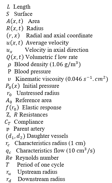
Nomenclature

1. Introduction

To date, the study of carotid artery disease remains crucial in the field of medicine and its allied globally. This disease predominantly occurs as a consequence of numerous risk factors. For example, low-density lipoprotein cholesterol, physical inactivity, genetic predisposition, obesity, diabetes mellitus etc, [1]. In severe circumstances, a plaque could rupture or break off, hence, sending parts of the obstruction to the brain arteries contributing to high blood pressure. When high blood pressure occurs, blood circulation halts beyond the edge of collapse, resulting in stroke. Therefore, monitoring high blood pressure whilst understanding its underlining factors is imperative to identifying tangible and feasible remedies for local, national, and global policies.

As revealed in the Lancet by the NCD Risk Factor Collaboration (NCD-RISC), the number of people with hypertension is over 1.28 billion globally in 2019 [2]. In Africa, this situation is no different as statistics have revealed a surge in the number of high blood pressure cases. About 82% out of the over 1.28 billion hypertension populace resides in Sub-Saharan Africa, low- and middle-income countries. Studies on high blood pressure cases can be dated back to the beginning of the 17th century. Although, a clearer understanding of the underlying principle regarding the dynamics of blood flow has not been fully realized, several authors have comprehensively researched into this field of study. Many of these studies primarily centred on the entire arterial systems whilst others focused on the circle of Willis.

2. Related Work

The model of [3] could delineate discontinuities and disruptions in blood flow, nevertheless could not provide prediction exactness of the pressure and flow patterns behavior. Siddiqui et al. [4] proposed Artificial Neural Network (ANN), Mamdani Fuzzy Inference System (MFIS) and Deep Machine Learning (DML) techniques to analyze cardiovascular diseases. Even though the DML model proposed is more accurate with a precision of 92.45% relative to the rest of the frameworks, however, the models could not capture the biological mechanisms of blood flow in the carotid artery. Flint et al. [5] performed a multivariable Cox survival analysis to determine the effect of the burden of systolic and diastolic hypertension on a composite outcome of myocardial infarction, ischemic stroke, or hemorrhagic stroke. Their findings however revealed systolic and diastolic hypertension independently predicted adverse outcomes, despite a greater effect of systolic hypertension. Mc Auley [6] employed the Ordinary Differential Equation (ODE) to model cardiovascular diseases. Despite their wide-spread applications, ODEs present several drawbacks. For example, it falls short when it is necessary to represent biological systems with more than one independent variable. Boolean models have also been utilized in the study of blood pressure and cardiovascular diseases [7]. Though their qualitative nature allows for representing gene networks, they are incapable of considering the biological mechanisms or enzyme kinetics. Dhange et al. [8] investigated blood flowing through an inclination pipe with stricture and expansion of a constant incompressible Casson model using a mild stenosis approximation technique.

3.0. Model description

It is alarming that cardiovascular diseases are plaguing the global population, and a clearer understanding of the pressure variations and flow is vital. This study employs the explicit finite difference method to investigate the key parameters of pressure variations in the human cranial arteries. In this section, we present the model description of the 1-D blood flow equations, taking into accounts the geometry, governing equations, boundary conditions and the numerical scheme used to solve the flow problem. The coefficients of viscosity of a fluid are shown to be Newtonian if they remain constant throughout all shear rates. Hence, since the artery diameters are huge compared to the individual cell diameters, it is fair to assume blood does have a constant viscosity in larger vessels. And, does the non-Newtonian behaviour become minimal, and blood can be regarded as a Newtonian fluid [9].

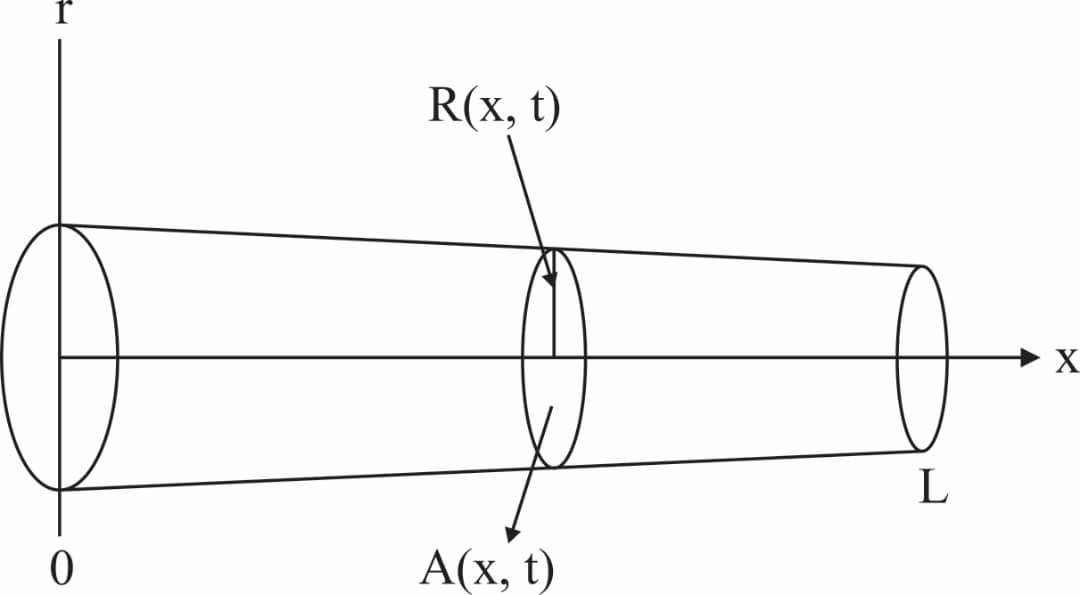
Consider blood as an incompressible fluid, flowing through an axisymmetric pressure cylinder with length L, surface S, area A(x,t), radius R(x,t), and (r,x) being the radial and axial coordinate respectively. The geometric view of the problem is seen in Figure 1. This geometry can be described using the 1-D Navier-Stokes equations in cylindrical coordinates as;

(1a)

According to [10], the no-slip condition and deformation of the elastic wall of the vessel allow for the boundary condition;

It is appropriate to define the area of cross-section,

and average velocity u(x,t), where u_x denote the velocity with constant in the axial direction as

The relationship between volumetric f low rate Q(x,t), and velocity, can then be express as

Following [10], and integrating over the cross-sectional area of Eq. (1a,1b) using the boundary condition Eq. 2 and the definitions (3a,3b,3c) gives;

where, (x,t) denote the axial and spatial coordinate along the artery, ρ the blood density, P represent the blood pressure, υ the kinematic viscosity and the flow of this study follows Poiseuille's law [11].

We obtain an underdetermine system, hence a third expression is needed to close the system. While some authors assume equilibrium at the start of the simulation and prefer P₀(x) as initial pressure, other models use other pressures, such as atmospheric pressure, to determine whether or not the artery is in the vertical position or treat it as a separate term P(x,t). [12], [13] assumed a thin wall tube based on linear elasticity where each section is independent of the others. Sochi [14] assume a linear pressure-area constitutive relation, where the pressure is proportional to arterial amplitude difference. Hence the third relation would provide a full mechanical model for the structure of the vessel wall. The deformation of the cranial artery after constriction is assume to be of the type A₀>A(x,t) and thus the tube law becomes

The system of mass momentum and continuity Eq. (4a,4b,4c), can be written in conservation form as;

where

Here, we denote r₀ the unstressed radius, A₀=πr₀² the reference area, and f(r₀)=4Eh/(3r₀) an expression for elastic response. Based on the compliance estimates of [15], [16], (Eh₀)/r₀=k₀ e^k₁r₀+k₂, where these constant estimates were given as k₀=2×10⁷ g.s^-2.cm^-1, k₁=-22.53 cm^-1 "and" k₂=8.65×10⁵ g.s^-2.cm^-1.

3.1 Boundary conditions

The above model suggests fluid pressure for a solitary cranial artery and thus boundary conditions are needed to truncate the computational domain. The inflow boundary condition at the inlet of the parent artery is specified by experimental data from [10]. The three element windkessel model has significant improvement over a purely resistive model [17] and hence was adopted as the outflow boundary condition.

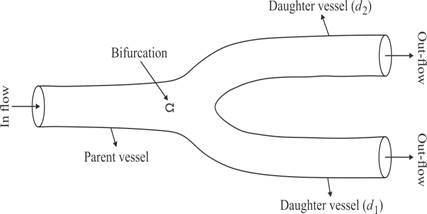
where Z,R represent the resistances and C_T compliance. The bifurcation indicates an outflow of the parent artery and the inflow of the daughter arteries, figure 2. Suppose from figure 2, that the bifurcation takes place at Ω, then the conservation of mass yields q_p(t)=q_d1(t)+q_d2(t) and p_p (t)=p_d1 (t)=p_d2(t), where p refers to the parent artery, left and right-daughter vessels as (d₁,d₂).

3.2. Dimensional analysis

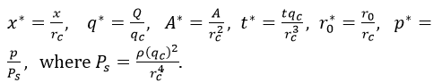
To analytically reduce the complexity of the fundamental equations describing the behaviour of the system, scaling analysis is performed to reduce the number of experimental parameters affecting the flow problem. With regards to our fluid flow equations presented by Eq. 5, we require to identify the set of parameters which characterize the behaviour of our system. Consider the following characteristics parameters: r_c=1 cm, the characteristics radius, ρ=1.06 g/m³, the density of the blood, q_c=10cm³/s, the characteristics flow. Now, if we scale the length to r_c and the flow to q_c, then it is obvious the area can be scale to r_c². Thus we obtain the following scaling quantities;

Now multiplying through Eq. 5 by r_c/q_c for the continuity equation, it satisfies

Similarly, multiplying through Eq. 5 by r_c³/q_c² , the momentum equation is written as,

where Re=q_c/vr_c is the Reynolds number.

If we suppress Eq. 7a and 7b, the scaled equations become

and the dimensionless Navier-Stokes equations can be written as

4.0. Numerical discretization

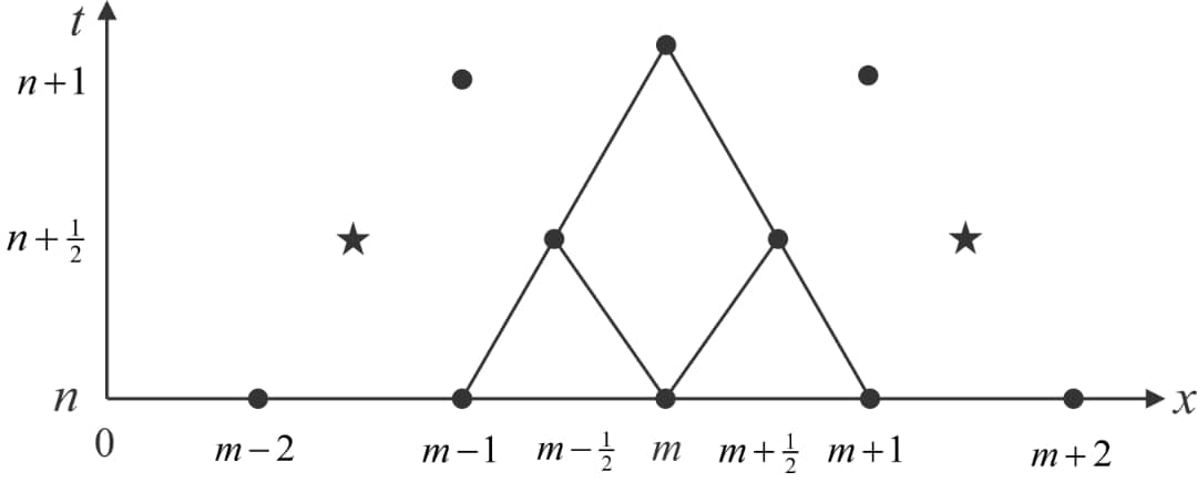
The numerical solution figure 3, follows an explicit finite difference scheme which is second order accurate in time and space [18]. We may write

We now consider U_mⁿ=U(mΔx,nΔt), the solution at nΔt time frame and position mΔx, where similar definitions can be made for H and E. Then, the flow q and area cross-section A at (n+1) is given as.

The n+1/2 time steps and m±1/2 position values of H and E for n+1/2 time interval can be found using

where j=m±1/2.

4.1. Inflow boundary conditions

This condition is applied at the entrance of the parent vessel of figure 2. The inflow q into the carotid artery necessitates the specification of flux values q(0,t). Using Newton's method, the value of A_0^(n+1) is determine by substituting q₀^n+1⁄2 into Eq. 9. The numerical scheme requires the estimated of;

4.2. Outflow boundary conditions

The outflow boundary condition, is applied at each of the outlet of figure 2 and is determine by the discretized three-element windkessel model as;

where Z,R represent the resistances and C_T compliance. Since the windkessel model is a function of q only, it requires the evaluation of pressure in the carotid artery, which is related to area A(x,t) via the discretized tube law Eq. 4c. Then using an iterative scheme with an initial guess for , the solutions for and is found, where as is calculated using Eq. 12. The algorithm stops at .

4.3. Bifurcation boundary conditions

The estimation of n+1/2 time steps and m±1/2 position values of H and E, allow for the introduction of imaginary points at the outlet of the parent artery and the inflow into the daughter arteries. Using these points, can be expressed as

where i=p,d₁,d₂, represents the parent, left, and right-daughter vessels respectively and m=M if i=p, otherwise m=0, given U=(A,q). Thus following [19], we assume conservation of flow and continuity of pressure as;

where U^*=(q,p) for r=(n+1/2,n+1). Taking the norm of Eq. 4c, the pressure continuity for r=(n+1/2,n+1),i=(d₁,d₂ ) is found as

(15)

Now the solution at t=n+1 time step for the parent and branching arteries in terms of flow rate and area cross-section is given as

and

From Eq. 13-17, we have a system of 18 nonlinear equations which can be solved using Newton’s iterative method

where g is the current iteration, x=(x¹,x²,…,x¹⁸),J(x^g ) is the Jacobian of the system of equations and f^g(x) are the residual equations. A Courant Friedrich's Lewy (CFL) stability threshold [20] dt/dx≤|u+c|^-1, where u is velocity (q⁄A) and c wave speed is used to fulfilled the stability of the numerical scheme. The accuracy of the results depends on the Lax-Wendroff method, which is analysed in terms of its order of convergence and stability. This method is second-order accurate in both time and space. Hence the global error E = O (Δt²+Δx² ). Next, the Courant-Friedrichs-Lewy (CFL) condition is met, and the method becomes stable.

Possible errors may arise from approximating the derivatives in the partial differential equations with finite differences. Since the method is second-order accurate, the truncation error is of the order stated above. Also, numerical dissipation can still occur due to round-off errors or if the time step is not chosen appropriately given the Lax-Wendroff method.

5. Simulation using the parameter values.

The simulations in this study were based on the set of parameters, of which the lengths and diameters were taken by magnetic resonance techniques and has been verified by the literatures; (Kolachalama et al. [15], Alastruey et al. [21], Olufsen et al. [16]). To avoid pressure buildup after each cycle, the values of the windkessel parameters of the outflow boundary condition are empirically estimated, whiles the density ρ = 1.06, period of one cycle, T = 0.917s and viscosity υ= 0.046 s^-1.cm² were adopted. As a result, four cardiac cycles were used for accuracy and precision of which the results are produced by our numerical approach.

Table 1. Physiological data obtained from Kolachalama et al. [15], Olufsen et al. [10], [16] representing length (L), upstream radius, r_u and downstream radius r_d.

	L (cm)	rd	ru
p	20.8	0.37	0.37
d1	17.7	0.28	0.29
d2	17.7	0.28	0.29

Figure 4a depicts the pressure in the carotid artery as a function of space  and time t, where all of the properties described by [10], [15], [16] can be found in the pressure profile. This signifies a good quantitative response between our results and the literature data. Thus, the systolic and diastolic pressures are similar to that of a normal subject. We have demonstrated the corresponding flow rate profile in Figure 4b, how the behaviour of wave propagation and reflection in the carotid artery separate from the incoming pulse wave and becomes more noticeable near the periphery.

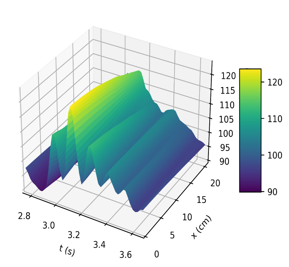
Modelling the dynamics of pressure and flow rate requires an understanding of the pulsatile nature of blood flow in the carotid artery. The elastic nature of the artery, the cardiac cycle, and other physiological variables all affect this dynamic process. Therefore, perturbation of these variables is required to examine changes in pressure and flow rate. As a result, we evaluate the model’s response to changes in these variables and the results can be seen in Figure 5 (a, b), Figure 6 (a, b), and Figure 7.

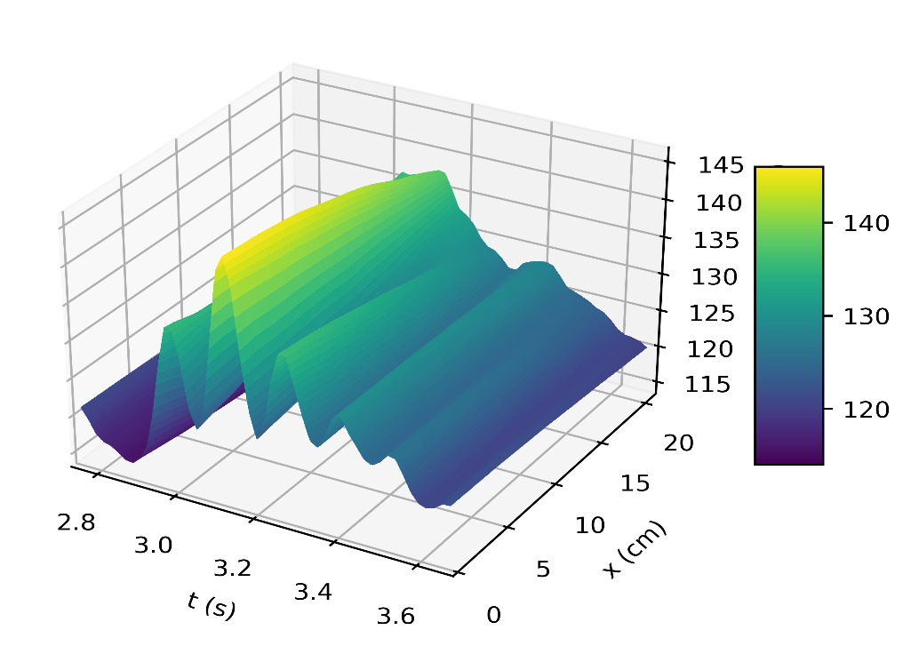
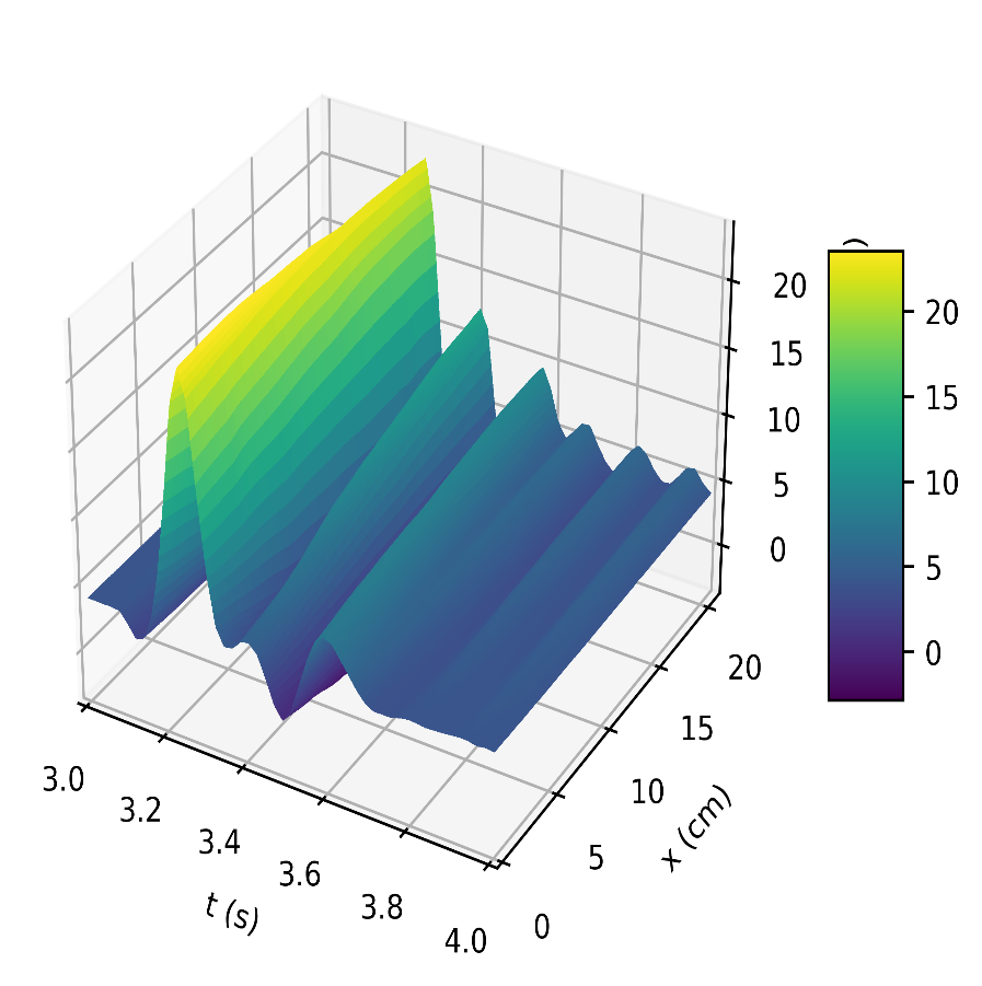
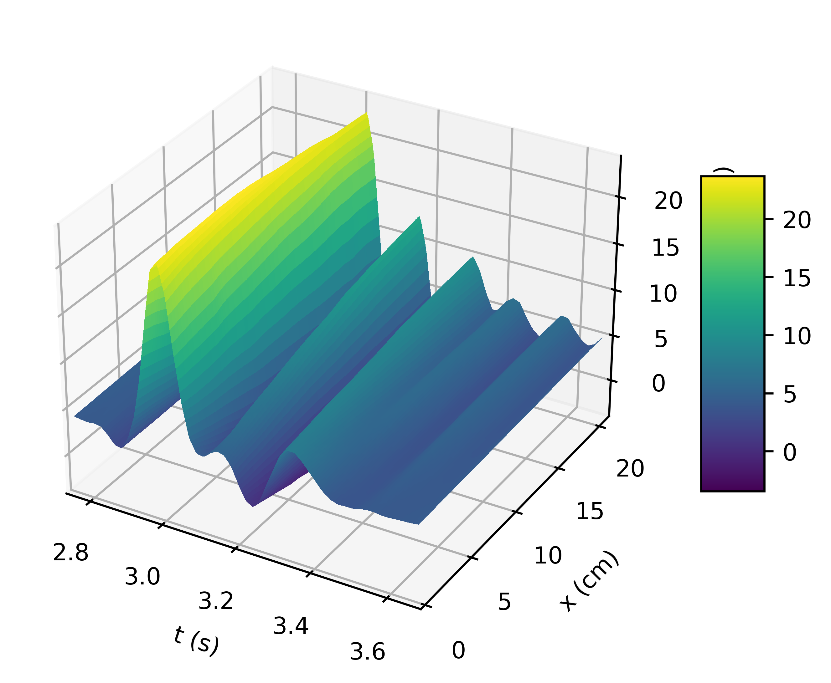
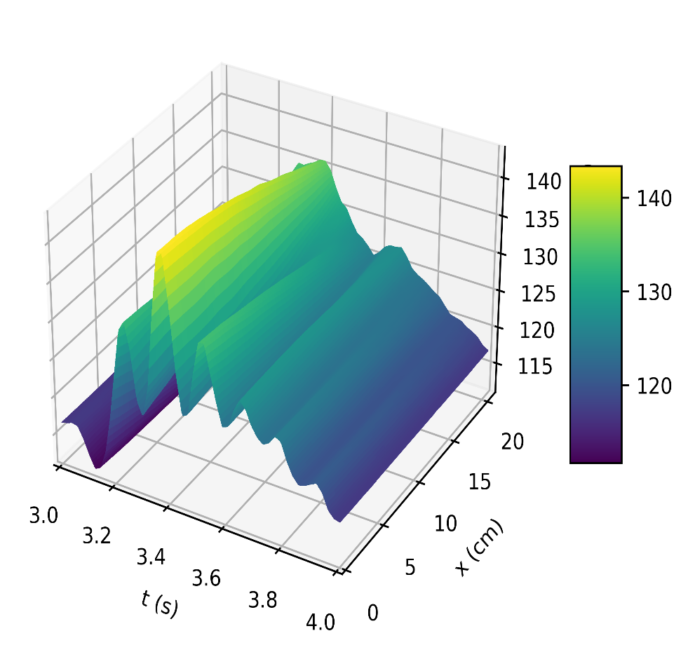
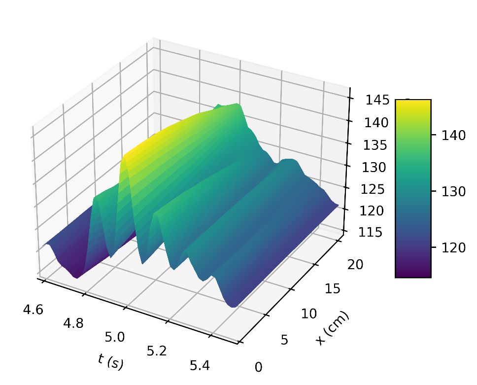
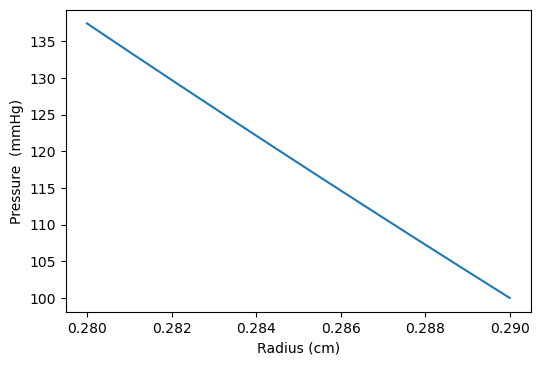
The results in Figures 5b, 6b, shows how the reflected waves separate from the incoming waves and become more noticeable near the periphery than at the proximal point. It can be seen from Figure 5a that, narrowing of the downstream radius has resulted in a high blood pressure situation since it has a systolic pressure of 140 mmHg or higher and diastolic pressure of 90 mmHg or higher [5]. Also, the reflected wave is layered on the incoming wave, increasing systolic pressure, which is the peak pressure during the cardiac cycle. Taking T =1s , where (r_u,r_d) remains the same as that for Figures 5a, 5b, it can be seen from Figure 6a the 0.083s increase in , has resulted in an increase in diastolic and a quite decrease in systolic pressure as a result of a slower heart rate. Figure 7 shows an increase in cardiac output to six, which results in an increase in diastolic and systolic pressures as there are more beats per minute, hence a higher heart rate. It is observed in the simulations that, the part of the wave with higher pressure travels faster to the periphery than the part with lower pressure. From Figure 8, we have illustrated, how a decrease in radius due to constriction results in a pressure increase, using the tube law equation from our model.

6. Conclusion

In this study, we examined a 1-D numerical simulation of the Navier-Stokes equations to investigate the dynamics of blood flow and pressure variations. A dimensional analysis was carried out, to reduce the complexity of the fundamental equations. Various boundary conditions were employed to ensure the model accurately represents the physical constraints and can better simulate the actual behaviour of the system, leading to more precise and reliable results.  Implementing appropriate boundary conditions helps to stabilize the numerical solution and ensures convergence of the model, particularly in complex 3D analyses. The resulting 1-D model was solved to determine flow and pressure at all points along the carotid artery using the explicit finite-difference method. Results were verified through the comparison with the available experimental data in the literature.

The results showed a rise in systolic and diastolic pulse pressure as we perturbed the parameters in our simulation, as seen in Figures 5a, 6a, and 7, and the peak flow diminished as we descended the peripheral cerebral bed. Also, a decrease in the radius of the cranial artery from (0.29-0.275)cm will result in the increase in pressure within the range (115mmHg-145mmHg) . In addition, the part of the wave with higher pressure travels faster to the periphery than the part with lower pressure.

References

[1] G. A. Roth, G. A. Mensah, C. O. Johnson, G. Addolorato, E. Ammirati, L. M. Baddour, N.C. Barengo, A. Z. Beaton, E.J. Benjamin, C. P. Benziger and A. Bonny, "Global Burden of Cardiovascular Diseases and Risk Factors, 1990-2019: Update From the GBD 2019 Study," Journal of the American College of Cardiology, vol. 76, no. 25. Elsevier Inc., pp. 2982-3021, Dec. 22, 2020. doi: 10.1016/j.jacc.2020.11.010. View Article
[2] A. E. Schutte, N. Srinivasapura Venkateshmurthy, S. Mohan, and D. Prabhakaran, "Hypertension in Low- and Middle-Income Countries," Circulation Research, vol. 128, no. 7. Lippincott Williams and Wilkins, pp. 808-826, Apr. 02, 2021. doi: 10.1161/CIRCRESAHA.120.318729. View Article
[3] B. Gutti, A. A. Susu, and O. A. Fasanmade, "Mathematical Modeling and Software Application of Blood Flow for Therapeutic Management of Stroke," Engineering, vol. 04, no. 04, pp. 228-233, 2012, doi: 10.4236/eng.2012.44030. View Article
[4] S. Y. Siddiqui, A. Athar, M. A. Khan, S. Abbas, Y. Saeed, M. F. Khan and M. Hussain, "Modelling, Simulation and Optimization of Diagnosis Cardiovascular Disease Using Computational Intelligence Approaches," J Med Imaging Health Inform, vol. 10, no. 5, pp. 1005-1022, Feb. 2020, doi: 10.1166/jmihi.2020.2996. View Article
[5] A. C. Flint, C. Conell, X. Ren, N. M. Banki, S. L. Chan, V. A. Rao, R. B. Melles and D. L. Bhatt, "Effect of Systolic and Diastolic Blood Pressure on Cardiovascular Outcomes," New England Journal of Medicine, vol. 381, no. 3, pp. 243-251, Jul. 2019, doi: 10.1056/nejmoa1803180. View Article
[6] M. T. Mc Auley, "Modeling cholesterol metabolism and atherosclerosis," WIREs Mechanisms of Disease, vol. 14, no. 3. John Wiley and Sons Inc, May 01, 2022. doi: 10.1002/wsbm.1546. View Article
[7] J. D. Schwab, S. D. Kühlwein, N. Ikonomi, M. Kühl, and H. A. Kestler, "Concepts in Boolean network modeling: What do they all mean?," Computational and Structural Biotechnology Journal, vol. 18. Elsevier B.V., pp. 571-582, Jan. 01, 2020. doi: 10.1016/j.csbj.2020.03.001. View Article
[8] M. Dhange, G. Sankad, R. Safdar, W. Jamshed, M. R. Eid, U. Bhujakkanavar, S. Gouadria and R. Chouikh, "A mathematical model of blood flow in a stenosed artery with post-stenotic dilatation and a forced field," PLoS One, vol. 17, no. 7 July, Jul. 2022, doi: 10.1371/journal.pone.0266727. View Article
[9] J. T. Ottesen, M. S. Olufsen, and J. K. Larsen, Applied Mathematical Models in Human Physiology. Society for Industrial and Applied Mathematics, 2004. doi: 10.1137/1.9780898718287. View Article
[10] M. S. Olufsen, C. S. Peskin, W. Y. Kim, E. M. Pedersen, A. Nadim, and J. Larsen, "Numerical Simulation and Experimental Validation of Blood Flow in Arteries with Structured-Tree Outflow Conditions," Ann Biomed Eng, vol. 28, no. 11, pp. 1281-1299, Nov. 2000, doi: 10.1114/1.1326031. View Article
[11] F. Liang, K. Fukasaku, H. Liu, and S. Takagi, "A computational model study of the influence of the anatomy of the circle of willis on cerebral hyperperfusion following carotid artery surgery," 2011. [Online]. Available: http://www.biomedical-engineering-online.com/content/10/1/84 View Article
[12] S. J. Sherwin, V. Franke, J. Peiró, and K. Parker, "One-dimensional modelling of a vascular network in space-time variables," J Eng Math, vol. 47, no. 3/4, pp. 217-250, Dec. 2003, doi: 10.1023/B:ENGI.0000007979.32871.e2. View Article
[13] J. Peiró, S. J. Sherwin, K. H. Parker, V. Franke, L. Formaggia, D. Lamponi and A. Quarteroni, "Numerical simulation of arterial pulse propagation using one-dimensional models."
[14] T. Sochi, "Flow of Navier-Stokes Fluids in Cylindrical Elastic Tubes," 2013.
[15] V. B. Kolachalama, N. W. Bressloff, P. B. Nair, and C. P. Shearman, "Predictive Haemodynamics in a One-Dimensional Human Carotid Artery Bifurcation. Part I: Application to Stent Design," IEEE Trans Biomed Eng, vol. 54, no. 5, pp. 802-812, May 2007, doi: 10.1109/TBME.2006.889188. View Article
[16] M. S. Olufsen, A. Nadim, and L. A. Lipsitz, "Dynamics of cerebral blood flow regulation explained using a lumped parameter model," Am J Physiol Regulatory Integrative Comp Physiol, vol. 282, pp. 611-622, 2002, doi: 10.1152/ajpregu. View Article
[16] D. L. Turcotte, J. M. Lyons, "A periodic boundary-layer flow in magnetohydrodynamics," J. Fluid Mech. 13(4), pp. 519-528, 1962. View Article
[17] S. Parragh, B. Hametner, and S. Wassertheurer, "Influence of an Asymptotic Pressure Level on the Windkessel Models of the Arterial System," IFAC-PapersOnLine, vol. 48, no. 1, pp. 17-22, 2015, doi: 10.1016/j.ifacol.2015.05.125. View Article
[18] T. K. Sengupta, V. K. Suman, S. Sengupta, and P. Sundaram, "Quantifying parameter ranges for high fidelity simulations for prescribed accuracy by Lax-Wendroff method," Comput Fluids, vol. 254, Mar. 2023, doi: 10.1016/j.compfluid.2023.105794. View Article
[19] B. N. Steele, D. Valdez-Jasso, M. A. Haider, and M. S. Olufsen, "Predicting arterial flow and pressure dynamics using a 1D fluid dynamics model with a viscoelastic wall," SIAM J Appl Math, vol. 71, no. 4, pp. 1123-1143, 2011, doi: 10.1137/100810186. View Article
[20] F. Amlani, N. Pahlevan, and N. M. Pahlevan, "A stable high-order FC-based methodology for hemodynamic wave propagation," J Comput Phys, vol. 405, 2020, doi: 10.1016/j.jcp.2019.109130ï. View Article
[21] J. Alastruey, K. H. Parker, J. Peiró, S. M. Byrd, and S. J. Sherwin, "Modelling the circle of Willis to assess the effects of anatomical variations and occlusions on cerebral flows," J Biomech, vol. 40, no. 8, pp. 1794-1805, 2007, doi: 10.1016/j.jbiomech.2006.07.008. View Article