Journal of Fluid Flow, Heat and Mass Transfer (JFFHMT)

ISSN: 2368-6111

Sensitivity of key Simulation Parameters on Flame Propagation in Obstructed Chamber: Effect of XiFOAM Discretization Schemes

Ayushi Mishra¹, Krishnakant Agarwal¹,Mayank Kumar¹

¹Indian Institute of Technology Delhi, Department of Mechanical Engineering
Hauz Khas, New Delhi, India 110016
ayushi.mishra@mech.iitd.ac.in; kkant@mech.iitd.ac.in; kmayank@mech.iitd.ac.in

Abstract - This paper uses the OpenFOAM Computational Fluid Dynamics (CFD) code to study the turbulent premixed flame propagation characteristics inside a partially open duct filled with obstacles. The simulations were performed using a two-dimensional model with realizable k-ε turbulence modelling and Flame Surface Density (FSD) model proposed by Weller et al. for Combustion modelling. The solver uses adaptive time stepping method coupled with a maximum value of the Courant number. Initially the simulations were carried out with first order upwind scheme for divergence terms, second order Crank Nicolson method for time discretization and PIMPLE solver (with outer correctors set to 200 with residual for outer correctors set to 10¬-4) for pressure-velocity coupling. The solution with these schemes resulted in impractical dependence of overpressure peak on the initial values of simulation parameters: turbulent kinetic energy ‘k’, initial time step size ‘Δt’, mesh size ‘Δx’ as well as maximum value for Courant number of the flow ‘maxCo’. The k values tested are 0.5, 0.1, 0.05 and 0.01, as at 0.01 the pressure peak was negligible and far delayed. Similar results have been obtained for above mentioned parameters. The discretization schemes were updated to a second order linear scheme for divergence terms and a first order Euler method for temporal terms. The pressure velocity coupling was updated to iterative PISO algorithm (PIMPLE in OpenFOAM, with outer correctors of three). The updated solver was then tested against the experimental results to analyse the dependence of pressure peak on the above-mentioned simulation parameters. It was found that the unexpected dependence on all the parameters was eliminated and the solver provided reasonably good qualitative agreement with the experimental results. Effect of each of the discretization schemes is also tested individually.

Keywords: XiFOAM, Discretization Schemes, Premixed Propagating Flames, Simulation Parameters.

© Copyright 2024 Authors - This is an Open Access article published under the Creative Commons Attribution License terms Creative Commons Attribution License terms. Unrestricted use, distribution, and reproduction in any medium are permitted, Pr ovided the original work is Pr operly cited.

Date Received: 2023-07-21
Date Revised: 2024-05-22
Date Accepted: 2024-06-10
Date Published: 2024-07-15

1. Introduction

Flame acceleration is an important phenomenon leading to explosions in chemical and mining industries [1]-[3]. As the flame gets ignited, the initial stage of flame propagation governs the extent of explosion, so therefore it is better to understand this part to mitigate the seriousness of the explosion. The mechanisms and models for flame acceleration have been studied for long to mitigate the explosion hazards and the possible onset of detonation [4]-[7]. In this study an attempt has been made to study the flame acceleration phenomena in partially open geometries, with obstacles, using the numerical approach. The XiFOAM solver available in OpenFOAM has been tested against the numerical results by Patel et al. [8].

Zhan Li et al. [9] used the XiFOAM solver of OpenFOAM to study gas explosions of methane-air mixtures in a large-scale tube with vents. The tube had a 0.8-meter cross-section and a 30-meter length. The LES k-equation model was used for turbulence modelling and the Weller model was used for combustion modeling. They came to the conclusion that vents might raise the flame traveling distance inside the tube and lower the peak pressure by 13% to 91%. Using the XiFOAM solver with Weller model, G. Luo et al. [10] investigated the effects of rectangular obstacle lengths on premixed methane–air flame propagation in a confined tube and found that the longer obstacles result in higher pressure because they provide ample acceleration time.

Yasari et al. [11] conducted an investigation into stationary premixed turbulent flames employing the XiFOAM solver. Similarly, Andreini et al. [12] examined XiFOAM, incorporating the Zimont model for stabilized lean premixed flames. Kutkan et al. [13] research also focused on stationary premixed turbulent flames using the XiFOAM solver, applying the standard k-ε model for turbulence and the Weller model for combustion modeling. Despite the numerous studies utilizing the XiFOAM solver, there is a notable gap in the literature regarding the influence of discretization schemes on the simulation outcomes for highly transient cases.

There has been limited research discussing in detail the impact of discretization schemes used in the XiFOAM solver, specifically in the context of Reynolds-Averaged Navier-Stokes (RANS) simulations of premixed flames propagating within partially open geometries with obstacles. As it is a highly transient phenomenon, the value of the pressure peak as well as its time of occurrence are two main parameters that should be well in agreement with the experimental results. The time here plays a crucial role in the simulations. Previous observations indicate that simulation results obtained with a specific set of discretization schemes are highly sensitive to initial simulation parameters. Key parameters exhibiting this dependence include the initial value of turbulent kinetic energy (k), the initial time step (Δt), the mesh size (Δx), and the maximum Courant number (maxCo). However, this dependency diminishes when different discretization schemes are employed. The study also examines the effects of various major discretization schemes, demonstrating that they significantly impact the simulation outcomes.

2. Methodology

2. 1. Combustion and Turbulence Model

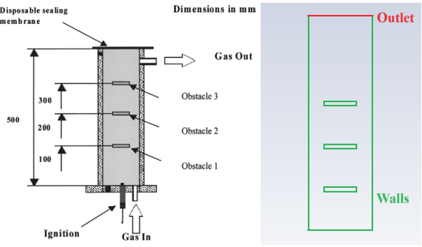
A two-dimensional planar model was selected to simulate the premixed flame propagation inside the obstructed chamber with 150×150×500 mm dimensions containing three centreline obstacles [8]. The experimental setup and the corresponding computational domain are shown in figure 1 (a) and (b) respectively. The premixed gas explosion reactions are a complex phenomenon involving chemical kinetics, heat transfer, and fluid dynamics. Under the assumption of simple one-step chemistry with the unity Lewis number and adiabatic conditions, the species transport equations can be reduced to a single combustion progress variable equation, as follows [14]

(1)

The progress variable in the above equation is described as,

(2)

where T is the temperature, and b stands for burned gas, and f stands for fresh gas. Here, c=0 implies burnt products and c=1 implies fresh fuel-air mixture.

To conduct the numerical simulations, CFD solver OpenFOAM has been used. In OpenFOAM, the XiFOAM solver is used to implement different flame surface density models. The XiFOAM solver instead of solving the transport equation for c, solves the transport equation for the regress variable b [15] which is defined as,

(3)

Hence the equation (1) can be re-written in terms of the regress variable b as follows,

(4)

In Equations (1) and (4), the overbar ¯ and the tilde ˜ refer to the Reynolds and Favre averaging, respectively. Here ρ is the density, α is the thermal diffusivity, μ_t is the turbulent viscosity, u is the flow velocity, S_u is the laminar flame speed, and S_ct is the turbulent Schmidt number.

Evaluating the mean reaction rate source term  in Equations (1) and (4) is the primary challenge in modeling premixed turbulent combustion. Both algebraic approaches [16], [17] and approaches based on extra transport equations [15] can be used to simulate this term. To validate the experimental results, this work employs a transport equation-based combustion model. The source term for the regress variable equation can be represented in the following way:

(5)

where ρ_u is the unburnt mixture density and the magnitude of the gradient term in Equation (5) can be evaluated as follows,

(6)

The turbulent flame speed , S_t appearing in Equation (5) is then modelled using the wrinkling factor, Ξ [18]

(7)

So, the source term becomes,

(8)

In case of Weller model [15], a transport equation is solved for the flame wrinkling factor. The transport equation is given as,

(9)

(10)

(11)

R_η is the Kolmogorov Reynolds number,  is the unstretched laminar flame speed, τ_η is the Kolmogorov time scale, while σ_s and σ_t represent the strain rates identified across the filtration surface, and u’ is the turbulent fluctuating velocity computed as

(12)

The transport equation for the laminar flame speed Su is employed in this manner.

(13)

where is the laminar flame speed at equilibrium conditions. In this model, the filtered laminar flame speed is expected to be transported at the strain rate time scale . This transport equation obeys the important constraints on the laminar flame speed.

The transport equation for the turbulent kinetic energy k and its dissipation rate ε was solved to get the turbulent viscosity using the realizable k-ε turbulence model [19]. The realizable model modifies the formulation of the turbulent viscosity ν_t and the transport equation for ε.

2. 2. Numerical Details

A two-dimensional computational model is tested with four different sizes of the hexahedral mesh elements, 1.5mm, 1mm, 0.75mm, and 0.5mm, giving a total number of elements as, 32,323, 72,926, 1,29,359, and 2,91,000 respectively. The initial and boundary conditions for the case are listed in table 1, four different values of initial turbulent kinetic energy are tested ranging from 0.5-0.01 m²/s².

For the numerical simulations using XiFOAM, the least-squares cell-based method was employed for gradient discretization. To prevent spurious oscillations, a multi-dimensional gradient limiter was utilized [20]. The convective terms in the governing equations were discretized with a limited linear scheme, which defaults to upwind in regions with rapidly changing gradients. The extent of upwinding in this scheme is controlled by a blending coefficient ranging from zero to one, where one represents aggressive limiting (upwinding) and zero indicates a pure linear scheme (highly accurate but prone to oscillations). The aforementioned discretization schemes were applied consistently in both the new and old sets of simulations.

The schemes that are updated in new discretization schemes are mentioned in table 2. The discretization scheme for the divergence terms used initially is the first order upwind scheme (limited linear with a limiting coefficient of one [21]), which is then updated to a second order central difference scheme (limited linear with a coefficient of zero) with corrections . This corrected numerical scheme for the diffusive terms takes into account mesh non-orthogonality and mesh stretching. The temporal term discretization scheme used earlier was the second order accurate Crank-Nicolson method which is then updated to first-order accurate Euler method and lastly the pressure-velocity coupling method was updated from PIMPLE, where 200 outer corrector steps were used, to iterative PISO with 3 outer corrector steps were used.

Table 1. Initial and Boundary Conditions

 

Variable	Description	Wall	Outlet	Internal Field
α	Turbulent Thermal Diffusivity	compressible::alphatWallFunction	calculated	0 kg/(m.s)
k	Turbulent Kinetic Energy	kqRWallFunction	zeroGradient	0.5-0.01 m2/s2
ε	Turbulent Kinetic Energy Dissipation Rate	epsilonWallFunction	zeroGradient	25 m2/s3
ν	Turbulent Viscosity	nutWallFunction	calculated	0 m2/s
b	Regress Variable	zeroGradient	zeroGradient	1
p	Pressure	zeroGradient	waveTransmissive	101.3kPa
Su	Laminar Flame Speed	zeroGradient	zeroGradient	0.35m/s
T	Temperature	zeroGradient	zeroGradient	293K
Tu	Unburnt Temperature	zeroGradient	zeroGradient	293K
U	Velocity	noSlip	zeroGradient	(0 0 0) m/s
Ξ	Flame Wrinkling Factor	zeroGradient	zeroGradient	1

Table 2 Updated Discretization Schemes

S.No	Discretization Term	Old Discretization Schemes	New Discretization Schemes
1	Divergence	First-Order Upwind	Second-Order Linear
2	Temporal	Second-Order Crank-Nicolson	First-Order Euler
3	Pressure-Velocity Coupling	PIMPLE	Iterative PISO

3. Results and Discussions

3. 1. Overpressure Plots with Old Discretization Schemes

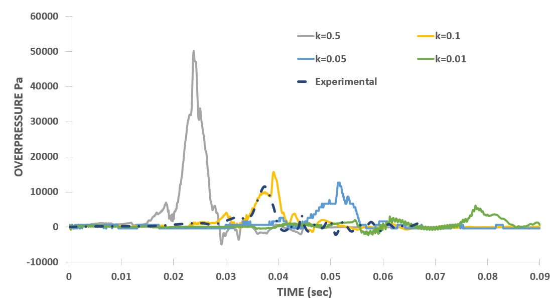
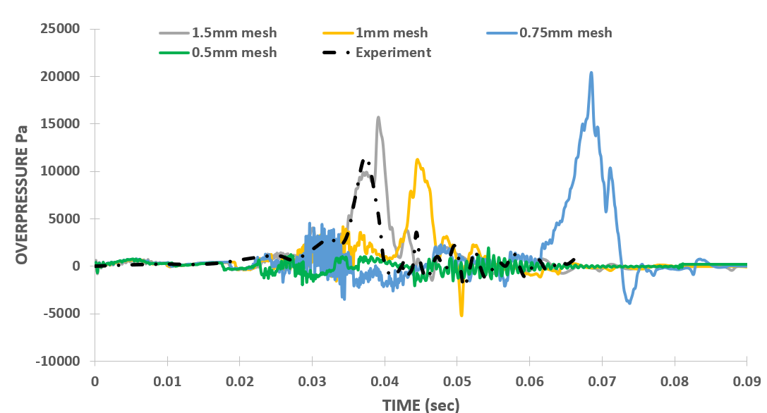
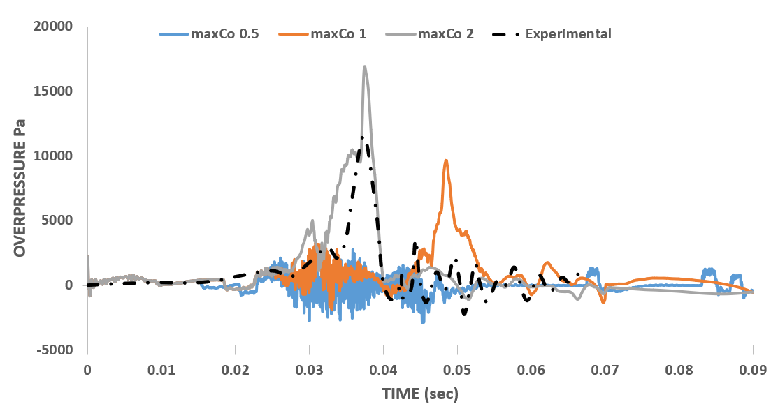
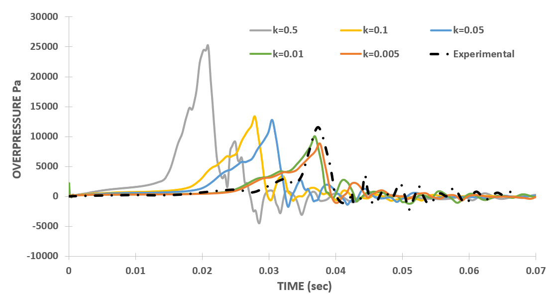
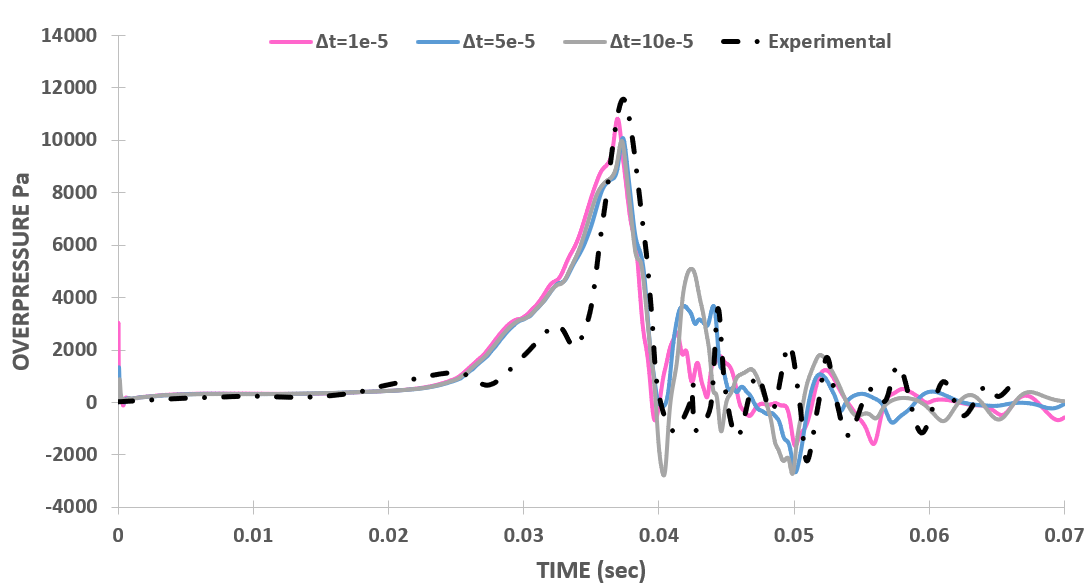
For validation with the experimental results, the overpressure inside the chamber is used as the initial and the most prior criteria. The overpressure is measured at the centre point of the bottom closed end of the chamber. This section presents overpressure plots with the old set of discretization schemes, figure 2 (a), (b), (c), and (d) represents the overpressure variation inside the chamber with k, Δt, Δx, and maxCo, respectively.

From Figure 2 (a), it is evident that the overpressure in the simulation exhibits a significant dependency on the initial turbulent kinetic energy (TKE), ‘k’ within the chamber. Notably, for a high 'k' value of 0.5, the overpressure reaches its peak at 50,205 Pa, approximately five times higher than the experimental value of 11,571 Pa. Conversely, a 'k' value of 0.1 yields a closer match to experimental results, peaking at 15,755 Pa with a time shift of 1.72 ms from the experiments. The percentage error in this case is 26.5%. Subsequent reduction of 'k' to 0.05 delays the overpressure peak to 51.4 ms, with a reduced peak value of 12,675 Pa. Further reduction to 'k' of 0.01 nearly abolishes the overpressure peak, registering only 6,185 Pa at 77.7 ms. Instances of absent or delayed pressure peaks coincide with flame stagnation, followed by re-initiation of propagation towards the chamber exit, as elaborated in Section 3. 3.

(a)

(b)

(c)

(d)

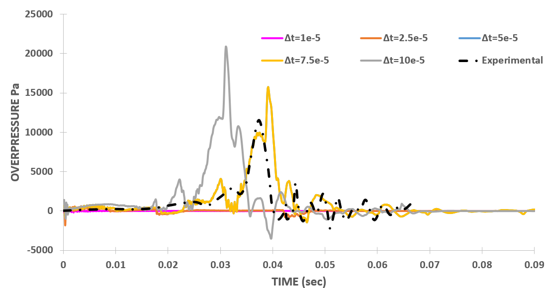
Figure 2 (b) illustrates the overpressure variations concerning the initial time step value, Δt. Despite employing an adaptive time-stepping method where Δt values dynamically adjust based on the maximum Courant number set in the case as the flow progresses, the results unexpectedly exhibit sensitivity to the initial Δt values. Five Δt values ranging from 10E^-5 to 1E^-5 are examined. Notably, for Δt value of 10E^-5 a premature overpressure peak occurs at 31 ms, reaching 20,865 Pa. Subsequent reduction of Δt initially shows convergence, with values of 7.5E^-5 and 5E^-5 yielding consistent results, peaking at 15,755 Pa at 39.1 ms, aligning reasonably well with experimental data. However, further reduction to 2.5E^-5 and 1E^-5 results in the absence of pressure peaks, halting flame propagation within the chamber entirely. This outcome contrasts expectations, as decreasing Δt values typically improve result accuracy.

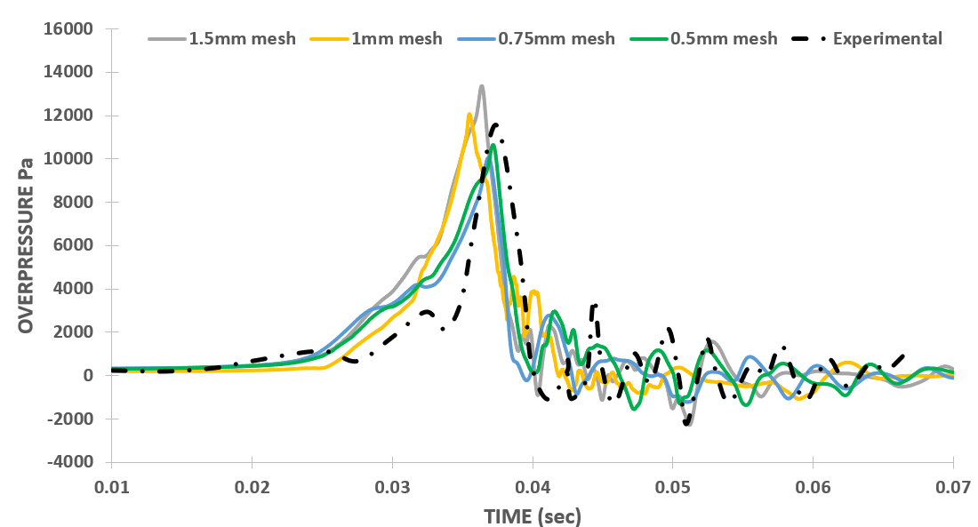
The effect of element size is analyzed in Figure 2 (c), where grid independence is tested. The mesh with a 1.5 mm element size showed good agreement with experimental data. However, refining the mesh, which is typically expected to enhance accuracy, led to deviations from the experimental overpressure results. Specifically, a mesh with a 1 mm element size resulted in a slightly delayed overpressure peak at 44.5 ms, reaching a value of 11,305 Pa. The plot indicates that a 0.75 mm element size caused a further delayed overpressure peak of 20,435 Pa at 68.4 ms. With further refinement to a 0.5 mm element size, no pressure peak was observed, and the flame became stagnant.

Analyzing Figure 2 (d) reveals a similar behavior in the overpressure plots with varying maximum values of the Courant number (maxCo). A maxCo value of 2 provided reasonable agreement with experimental results, showing an error of 26.5%. However, contrary to expectations that reducing maxCo would improve accuracy, the plots demonstrated a different trend. For a maxCo value of 1, the overpressure peak was delayed to 48.5 ms, with a peak value of 9,682 Pa. Further reducing maxCo to 0.5 resulted in the overpressure peak disappearing entirely.

With this set of discretization schemes, the overpressure plots exhibited consistent behavior with variations in all simulation parameters. This behavior, unexpected from a CFD perspective, was nonetheless consistent across different parameters. For instance, reducing the turbulent kinetic energy (k) value delayed the overpressure peak, a trend also observed when reducing the initial time step (Δt), mesh size (Δx), and maxCo values. Essentially, refining the case disrupted the flame propagation over time, indicating the critical role of the relationship between time stepping and space stepping in such highly transient simulations.

(a)

(b)

(c)

(d)

A specific configuration, with k=0.1, Δt=5E-5, Δx=1.5 mm, and maxCo=2, yielded reasonable agreement with experimental results, showing a 26.5% error and a time shift of 1.72 ms. However, altering any of these parameters disrupted the balance between time stepping and space stepping, resulting in slower flame propagation or complete failure of flame propagation in certain cases.

3. 2. Overpressure Plots with New Discretization Schemes

This section presents the overpressure variation with simulation parameters implemented with new set of discretization schemes. Figure 3 (a), (b), (c), and (d) illustrate the overpressure plots with the variation in ‘k’, ‘Δt’, ‘Δx’, and ‘maxCo’ respectively.

From Figure 3 (a), it is evident that the overpressure peak and its time of occurrence depend on 'k' values, which aligns with expectations. A higher initial 'k' value results in increased turbulence within the chamber, causing the flame to propagate faster. Then as 'k' values decrease, the overpressure peak value reduces correspondingly. The simulation results are well-validated against experimental data for 'k' = 0.01, showing an overpressure peak of 10,061 Pa at 36.84 ms, with a time shift of only 0.54 ms from experiments and a 13% error in the peak value. Testing with 'k' = 0.005 yielded similar results, indicating that the simulations are independent of the initial 'k' value inside the chamber.

Figure 3 (b) displays overpressure plots for different initial 'Δt' values. With the new discretization schemes, the results are independent of the initial value of 'Δt' as for three different values the overpressure plots are essentially the same in terms of overpressure peak value and its time of occurrence. The overpressure peak is 10,830 Pa at 36.94 ms, with a 6.4% error and a 0.44 ms time shift from the experimental peak.

The figure 3 (c) shows the dependence of overpressure plot on the grid size of the mesh, ranging from the coarsest mesh (1.5 mm) to the finest mesh (0.5 mm). The results indicate that with the new discretization schemes, grid independence has been successfully achieved. All grid sizes agree reasonably with experimental results, establishing an appropriate relationship between space stepping and time stepping. The meshes of 0.75 mm and 0.5 mm are particularly close, with errors of 13% and 7.97%, and time shifts of 0.5 ms and 0.2 ms, respectively. Therefore, a mesh size of 0.5 mm can be used for further simulations.

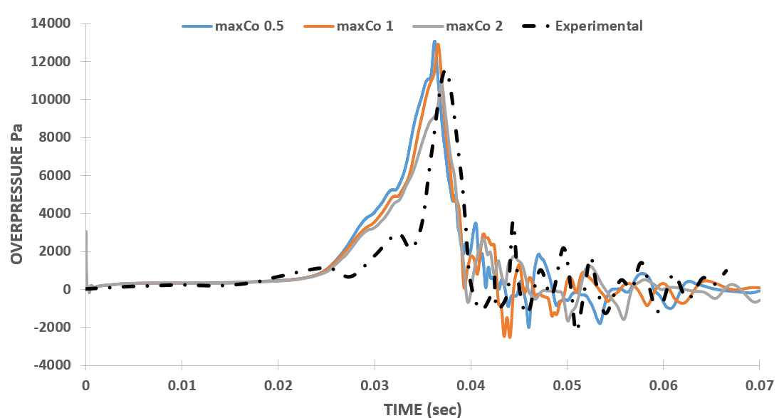
Figure 3 (d) shows the variation of overpressure plots with different values of maximum Courant number ‘maxCo’ of the case. The graph indicates that the unexpected dependence of overpressure results on ‘maxCo’ has also been eliminated by updating the discretization schemes. Thus, it can be concluded that the results, initially very sensitive to simulation parameters, are now, through changes in three discretization schemes, not unexpectedly dependent on these parameters. This update has achieved good agreement with experimental results across different ranges of these simulation parameters and for k=0.01 and Δt=1E^-5 the numerical results are well validated against the experimental results (figure 3 (a) and (b)).

3. 3. Flame Contours Comparison

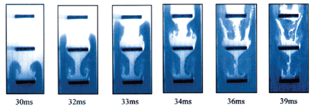
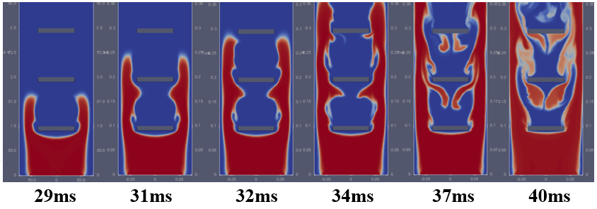
This section validates  the simulation results with new schemes by comparing the flame contour images for the three cases: experimental [8](figure 4 (a)), simulation results with new set of discretization schemes and with simulation parameters as, k = 0.01, Δt = 1E^-5, Δx = 0.5mm, and maxCo = 1 (figure 4 (b)), simulation results with old set of discretization schemes and with simulation parameters as, k = 0.01, Δt = 1E^-5, Δx = 1.5mm, and maxCo = 1 (figure 4 (d)). Figures 4 (c), and (e) show the corresponding overpressure plots for the flame contours given in figures 4 (b), and (d) respectively, to relate the flame propagation and the overpressure plot generated correspondingly.

Comparing the simulation results (figure 4 (b) and (c)) with new set of discretization schemes and above-mentioned parameters, with the experimental results by Patel et al. [8] (figure 4 (a)), it is concluded that the numerical results are very well validated against the experimental results with a percentage error of 6.4% in the peak overpressure value and a time shift of only 0.44 ms. The flame contours have also shown a decent match with the experiments in terms of lateral and transverse propagation of the flame within their respective timing.decent match with the experimental images of the flame contours in terms of lateral propagation of the flame. In figure 4 (c) the numerical results with k = 0.01, Δt = 1E^-5, Δx = 0.5mm, and maxCo = 1

(a)

(b)

(c)

(d)

(e)

In figure 4 (d) where old discretization schemes were used, the flame became stagnant after reaching close to the first obstacle for about 30-40ms. From the start also the flame propagation was slower compared to the experimental case, as at 30ms the flame had not yet reached the first obstacle whereas in experimental results the flame had already crossed it by this time. So, the propagation of the flame with older schemes has failed, as the flame finds it difficult to propagate from one cell to the other under certain conditions of the simulation parameters.

The older schemes only provided reasonable agreement with the experiments when using parameters k = 0.1, Δt = 7.5E-5, Δx = 1.5 mm, and maxCo = 2. Any changes to these parameters resulted in the flame either failing to propagate (remaining stagnant throughout the simulation) or experiencing delays or advancements. This highlights the crucial role of the coupling between time stepping and space stepping for highly transient cases.

3. 4. Effect of each Discretization Scheme

As outlined in Table 2, a total of three discretization schemes were updated in the new set of schemes. This section will separately analyze the effect of each discretization scheme using a mesh size of 1.5 mm and two extreme values of 𝑘, namely 𝑘 = 0.5 and 𝑘 = 0.01. While testing each scheme, the other two discretization schemes mentioned in Table 2 were updated to their new versions. For example, while testing the temporal discretization, only the temporal term uses the Crank-Nicolson method, whereas the divergence term and pressure-velocity coupling are updated to second-order linear and iterative-PISO, respectively.

Figure 5 (a), (b), and (c) illustrate the effects of divergence term discretization scheme, temporal discretization scheme, and pressure-velocity coupling mechanism, respectively. There are two parameters considered for the comparison of three different discretization schemes, first, the time difference in both the peak and second, the difference in peak overpressure values. Both parameters are shown in table 3. From this table, it can be concluded that the maximum values for both of these parameters are for the temporal term, the Crank-Nicolson method. Therefore, the Crank-Nicolson method has the most significant effect on the simulation results, being highly sensitive to the simulation parameters. The next notable impact is attributed to the pressure-velocity coupling method. Therefore, updating from PIMPLE to iterative PISO method has also greatly the results. The least effect is observed in the divergence term discretization.

The Crank Nicolson method due to its diffusive nature and difficulty in accurately resolving the discontinuity failed to capture the propagating flame. This method, characterized by its implicit time integration scheme, tends to diffuse abrupt changes in the solution over time steps, leading to smearing of discontinuities and blurring of sharp features such as flame front represents a sharp discontinuity in temperature and species concentrations, the Crank-Nicolson method struggles to accurately capture the dynamics of the flame propagation.

(a)

(b)

(c)

Table 3. Comparison of three Discretization Schemes Separately

Discretization Term	Time between two peaks (ms)	Difference in peak values (Pa)
Divergence	16.75	14,919
Temporal	46.17	42,492
Pressure-Velocity Coupling	25.28	38,396

4. Conclusion

This study focuses on the simulation of turbulent premixed flame propagation in a chamber with three centreline obstacles. The OpenFOAM Computational Fluid Dynamics (CFD) code with a two-dimensional planar model is used to simulate the complex phenomenon of gas explosion reactions. Initially, the simulations were carried out with first order upwind scheme for divergence terms, second order Crank Nicolson method for time discretization, and PIMPLE solver for pressure-velocity coupling. The solution with these schemes resulted in impractical dependence of overpressure peak on the initial values of simulation parameters: turbulent kinetic energy (k), initial time step size (Δt), mesh size (Δx), and maximum value for Courant number of the flow (maxCo). In this case, only some particular values of simulation parameters produced results that matched the experimental results closely, minor changes to any single parameter were causing drastic and unexpected deviations. The discretization schemes were updated to a second order linear scheme for divergence terms and a first order Euler method for temporal terms. The pressure velocity coupling was updated to an iterative PISO algorithm. The updated solver was tested against the experimental results to analyze the dependence of pressure peak on the above-mentioned simulation parameters.

The study presents overpressure plots with old and new discretization schemes for validation with experimental results. The results show that the overpressure in the simulation exhibits a significant dependency on the initial turbulent kinetic energy (TKE), 'k' within the chamber. The results unexpectedly exhibit sensitivity to the initial Δt values, despite employing an adaptive time-stepping method. The effect of element size, and maximum values of the Courant number (maxCo) also show inconsistent behavior with variations in all simulation parameters.

The new discretization schemes show that the overpressure peak and its time of occurrence depend on 'k' values, which aligns with expectations. The simulation results are well-validated against the experimental data for 'k' = 0.01, showing an overpressure peak of 10061 Pa at 36.84 ms, with a time shift of only 0.54 ms from experiments and a 13% error in the peak value. The new discretization schemes successfully achieve grid independence, establishing an appropriate relationship between space stepping and time stepping. The unexpected dependence of overpressure results on maxCo has also been eliminated by updating the discretization schemes.

This study compares flame contour images from experimental, simulation results with new discretization schemes, and old schemes. The simulation results show a decent match with experimental flame contours in terms of lateral propagation. However, the flame propagation with older schemes failed due to the flame's difficulty in propagating from one cell to another under certain simulation parameter conditions. The coupling between time stepping and space stepping is crucial for highly transient cases. The Crank-Nicolson method struggles to accurately capture the dynamics of flame propagation when applied to simulations involving propagating flames, where the flame front represents a sharp discontinuity in temperature and species concentrations. The method's diffusive nature and difficulty in accurately resolving discontinuities lead to smearing of discontinuities and blurring of sharp features such as flame fronts.

References

[1] "It's Not Just Vizag And Bhopal: Past Major Gas Leaks In India," 2020. View Article
[2] E. Advisors, "WorkOSH Major Industrial Disasters in India," vol. 9, no. 4, pp. 1-8, 2014.
[3] H. Yang, J. Chen, H. Chiu, and T. Kao, "Kaohsiung Vapour Explosion - A Detailed Analysis of the Tragedy in the Harbour City," vol. 48, pp. 721-726, 2016, doi: 10.3303/CET1648121.
[4] V. Di Sarli, A. Di Benedetto, G. Russo, S. Jarvis, E. J. Long, and G. K. Hargrave, "Large eddy simulation and piv measurements of unsteady premixed flames accelerated by obstacles," Flow, Turbul. Combust., vol. 83, no. 2, pp. 227-250, 2009, doi: 10.1007/s10494-008-9198-3. View Article
[5] S. R. Gubba, S. S. Ibrahim, W. Malalasekera, and A. R. Masri, "An assessment of large eddy simulations of premixed flames propagating past repeated obstacles," Combust. Theory Model., vol. 13, no. 3, pp. 513-540, 2009, doi: 10.1080/13647830902928532. View Article
[6] O. Vermorel, P. Quillatre, and T. Poinsot, "LES of explosions in venting chamber: A test case for premixed turbulent combustion models," Combust. Flame, vol. 183, pp. 207-223, 2017, doi: 10.1016/j.combustflame.2017.05.014. View Article
[7] P. Chen, Y. Sun, Y. Li, and G. Luo, "Experimental and LES investigation of premixed methane/air flame propagating in an obstructed chamber with two slits," J. Loss Prev. Process Ind., vol. 49, pp. 711-721, 2017, doi: 10.1016/j.jlp.2016.11.005. View Article
[8] S. N. D. H. Patel, S. Jarvis, S. S. Ibrahim, and G. K. Hargrave, "An experimental and numerical investigation of premixed flame deflagration in a semiconfined explosion chamber," Proc. Combust. Inst., vol. 29, no. 2, pp. 1849-1854, 2002, doi: 10.1016/S1540-7489(02)80224-3. View Article
[9] Z. Li et al., "Gas explosions of methane-air mixtures in a large-scale tube," Fuel, vol. 285, no. August 2020, p. 119239, 2021, doi: 10.1016/j.fuel.2020.119239. View Article
[10] G. Luo, J. Tu, and Y. Qian, "Impacts of Rectangular Obstacle Lengths on Premixed Methane - Air Flame Propagation in a Closed Tube," vol. 58, no. 1, pp. 10-21, 2022, doi: 10.1134/S0010508222010026. View Article
[11] E. Yasari, S. Verma, and A. N. Lipatnikov, "RANS Simulations of Statistically Stationary Premixed Turbulent Combustion Using Flame Speed Closure Model," Flow, Turbul. Combust., vol. 94, no. 2, pp. 381-414, 2015, doi: 10.1007/s10494-014-9585-x. View Article
[12] A. Andreini, C. Bianchini, and A. Innocenti, "Large Eddy Simulation of a Bluff Body Stabilized Lean Premixed Flame," vol. 2014, 2014. View Article
[13] H. Kutkan and J. Guerrero, "Turbulent premixed flame modeling using the algebraic flame surface wrinkling model:A comparative study between openFOAM and ansys fluent," Fluids, vol. 6, no. 12, 2021, doi: 10.3390/fluids6120462. View Article
[14] R. K. Shah and A. L. London, Laminar Flow Forced Convection in ducts, Supplement 1 to Advances in Heat Transfer. New York: Academic Press, 1978. View Article
[14] V. Zimont, W. Polifke, M. Bettelini, and W. Weisenstein, "An efficient computational model for premixed turbulent combustion at high reynolds numbers based on a turbulent flame speed closure," Proc. ASME Turbo Expo, vol. 2, no. July 1998, 1997, doi: 10.1115/97-GT-395. View Article
[15] H. G. Weller, G. Tabor, A. D. Gosman, and C. Fureby, "Application of a flame-wrinkling les combustion model to a turbulent mixing layer," Symp. Combust., vol. 27, no. 1, pp. 899-907, 1998, doi: 10.1016/S0082-0784(98)80487-6. View Article
[16] V. L. Zimont and A. N. Lipatnikov, "A Model of Premixed Turbulent Combustion and its Validation," Chem. Phys. Reports, vol. 120, no. January 1994, pp. 993-1025, 1995.
[17] S. P. Reddy Muppala, N. K. Aluri, F. Dinkelacker, and A. Leipertz, "Development of an algebraic reaction rate closure for the numerical calculation of turbulent premixed methane, ethylene, and propane/air flames for pressures up to 1.0 MPa," Combust. Flame, vol. 140, no. 4, pp. 257-266, 2005, doi: 10.1016/j.combustflame.2004.11.005. View Article
[18] T. Schmitt, M. Boileau, and D. Veynante, "Flame wrinkling factor dynamic modeling for large eddy simulations of turbulent premixed combustion," Flow, Turbul. Combust., vol. 94, no. 1, pp. 199-217, 2015, doi: 10.1007/s10494-014-9574-0. View Article
[19] S. T.H., L. W.W., S. A., Y. Z., and Z. J., "A new k-ϵ eddy viscosity model for high reynolds number turbulent flows," in Computers and Fluids, 1995, pp. 105-116. doi: 10.1016/0045-7930(94)00032-T. View Article
[20] S. Kim, B. Makarov, and D. Caraeni, "A Multidimensional Linear Reconstruction Scheme for Arbitrary Unstructured Grid," in In Proceedings of the AIAA 16th Computational Fluid Dynamics Conference, Orlando, FL, USA,
[21] E. Robertson, V. Choudhury, S. Bhushan, and D. K. Walters, "Validation of OpenFOAM numerical methods and turbulence models for incompressible bluff body flows," Comput. Fluids, vol. 123, pp. 122-145, 2015, doi: 10.1016/j.compfluid.2015.09.010. View Article