Journal of Fluid Flow, Heat and Mass Transfer (JFFHMT)

ISSN: 2368-6111

Parametric Study on Enhanced Thermal Management via Regulated Impingement Boiling Cooling

Djamel E Guerfi^1,2, Stéphane Roux³, Nadine Allanic², Alain Sarda ², Damien Lecointe ¹

¹Nantes Université, IRT Jules Verne, F-44000 Nantes, France
djamel-eddine.guerfi@etu.univ-nantes.fr; damien.lecointe@irt-jules-verne.fr
²Nantes Université, CNRS, GEPEA, UMR 6144, F-44000 France
nadine.allanic@univ-nantes.fr; alain.sarda@univ-nantes.fr
³Nantes Université, CNRS, Laboratoire de thermique et énergie de Nantes, LTeN, UMR 6607, F-44000 Nantes, France
stephane.roux@univ-nantes.fr

Abstract - This study comprehensively investigates impinging jet cooling mechanisms within a thermal regulation framework. Utilizing an innovative cooling approach based on the Smart Element of Cooling with impinging jets and transverse airflow, a 3D numerical model based on the Inverse Heat Conduction Problem (IHCP) is developed. This model quantifies heat exchange distribution at the wall of a confined cylindrical space with a margin of error below 3%. The study demonstrates the effectiveness of a regulation algorithm in maintaining target cooling rates, highlighting significant influences of jet aerodynamic and hydraulic parameters, such as flow rate ratios, jet orientation, size, and distribution on cooling performance. The research aims to define the optimal jet configuration for efficient heat dissipation while maintaining precise temperature control and enhanced cooling uniformity. Optimal configurations are found to depend on desired cooling rates and ratio combinations. For average cooling rates around 15°C/min, a spacing ratio of 30 between jets, a hydraulic diameter ratio of 7.5, and a flow ratio of 4 appear optimal for achieving enhanced cooling uniformity. These configurations present promising prospects for designing more efficient cooling systems in various industrial applications, thereby enhancing manufacturing process performance.

Keywords: Jet Impingement Boiling, Enhanced Thermal Management, Cooling Regulation, Heat Transfer Optimization, Multiphase Flow.

© Copyright 2024 Authors - This is an Open Access article published under the Creative Commons Attribution License terms Creative Commons Attribution License terms. Unrestricted use, distribution, and reproduction in any medium are permitted, Pr ovided the original work is Pr operly cited.

Date Received: 2023-10-06
Date Revised: 2024-05-17
Date Accepted: 2024-05-29
Date Published: 2024-06-28

1. Introduction

The utilization of jets for mold cooling is prevalent in various industrial applications [1-2]. This technique has demonstrated its efficacy in maintaining optimal temperatures in sectors such as the aerospace industry and sheet metal production. However, in the processing of advanced thermoplastic matrix composite materials, high processing temperatures up to 400°C are sometimes required. These temperatures can induce convective boiling phenomena and cooling inconsistencies, potentially compromising the quality of the produced parts [3]. Compression molding, which involves a preheating phase followed by a cooling phase, is a common method for shaping these materials, making thermal management crucial. Agazzi et al. [4] provided a comprehensive review of the thermal influences on the final state of composite parts, identifying several phenomena that can impact process quality. Lin also investigated the effects of reduced cooling times on the quality of formed components [5]. Non-uniform or excessively rapid cooling can result in issues such as uncontrolled part shrinkage and cracking [6-7]. Furthermore, improper cooling can cause defects in components, including deformation, shrinkage, residual thermal stresses, and indentation marks [8]. Thus, the cooling phase significantly affects both productivity and the quality of manufactured parts [9].

2. Related Work

To produce high-quality components and overcome limitations associated with traditional configurations of channels connected in parallel or series, controlled and homogeneous cooling has become essential. Various techniques have been developed to enhance thermal management, including the design of composite forming tools with lattice structures, optimization of conformal cooling channels (CCC), and the rapid thermal cycle molding (RHCM) approach characterized by electrical heating and annular cooling. Research has also focused on the effects of heat flux density on the heterogeneity of water phases along channels [10-12].

The assessment of heat exchange in cooling by jet impact is an evolving research field. Reviews have addressed the dependence of thermal flux density on factors like jet velocity, total mass flow rate, and jet diameter [13-14]. Optimal spacing between jets to ensure efficient heat transfer, particularly in overlapping zones, has also been explored [15]. Studies on the cross-flow of transverse air with water jets have identified optimal flow conditions and jet stability thresholds [16]. The effects of Reynolds number and nozzle-to-surface distance on heat exchange, as well as the interaction between neighbouring jets, have been investigated to determine the highest heat transfer coefficients in overlap zones [17-18].

Novel theoretical frameworks to forecast critical heat flux (CHF) in microchannels have been introduced, considering factors such as fluid type, saturation temperature, mass flux, and microchannel characteristics [19]. Visualization of two-phase flow and distribution of water phases during the cooling of heated cylindrical channels has highlighted the dependence of heat exchange on gradients and vapor volume fractions [20].

Building on previous research, an innovative approach developed at the laboratory using boiling induced by impacting jets combined with transverse airflow aims to achieve uniform and controlled cooling, improving thermal management and part quality. Subsequent studies revealed that introducing air between hot water jets and a concave surface increased the wetted area and enhanced heat transfer significantly. The development of the Smart Element of Cooling (SEC) concept directs water flow perpendicular to the channel surface, minimizing heterogeneities due to phase changes along the channels, thus enhancing thermal management [21-22].

The objective of this work is to evaluate the influence of parameters such as fluid flow rate ratio, jet orientation, number, spacing, and diameter on the cooling rate of the upper surface in contact with the machined part, the uniformity of cooling, as well as heat exchange with cylindrical channel walls. Despite extensive research, no existing studies have examined boiling cooling processes with multiple jets in the presence of cross-flowing air in a confined cylindrical space.

In summary, this study seeks to better understand multi-phase heat transfer in cooling channels with water jets subjected to cross-flowing air, contributing to advancements in thermal management and component quality in composite material processing.

3. Experiment and methods

3. 1. Description of the Experimental Setup

The experimental setup, as illustrated in Figure 1, includes fluid conduits and the test element, which is a 316L stainless steel block measuring 200 mm × 100 mm × 90 mm. An upstream quartz tube directs air to the entrance of the central perforated channel in the block which has a diameter of 27 mm. , while the downstream tube carries the water/air/steam mixture. A central tube, coaxially inserted into the perforated channel, generates water jets by directing all the water to the orifices at the end of the tube.

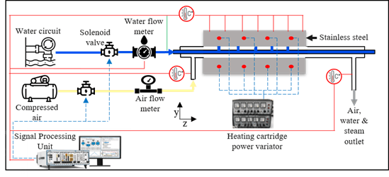
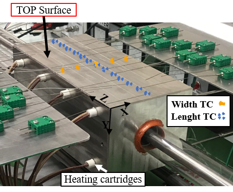
The test element is heated to 320 °C using eight heating cartridges (Figure 2). A low air flow rate of 14 l/min is maintained in the annular space between the tube and the channel surface to evacuate water vapor and prevent condensation. Once the test element reaches an average temperature of 300 °C, as measured by 25 type K thermocouples (0.5 mm diameter) on its top surface (Figure 2), the cooling process begins with the activation of the water jets.

Cooling uniformity along the length of the test element is assessed using 13 thermocouples indicated in blue in Figure 2 , while uniformity along the width is measured with five thermocouples indicated in orange in Figure 2.

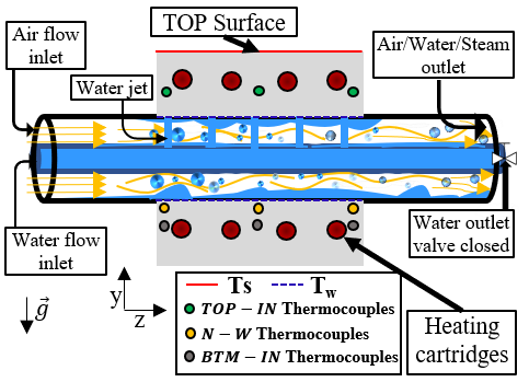
Additionally, nine type K thermocouples (3 mm diameter) are inserted into the steel block: six placed 15 mm from the wall, three on each side, with upper thermocouples in green and lower ones in grey in Figure 3 and three near-wall thermocouples positioned 5 mm from the wall in the lower part, indicated in yellow in Figure 3.

The steel block is insulated with a 20 mm layer of AES wool (synthetic fibers, alk. earth silicate) with low thermal conductivity (0.048 W·m^-1·K^-1 to minimize temperature losses and mitigate natural convection effects. This insulation significantly improves thermal performance, reducing the natural cooling rate from 3 to 1 °C/min.

3. 2. Cooling control procedure

Once the average temperature of the 25 thermocouples on the upper surface reaches 300°C, the cooling process by impacting jets is initiated with a binary cooling process, wherein the algorithm compares the average cooling rate with the Target Cooling Rate (TCR). Based on this comparison, the jets are either activated or deactivated.

Throughout the entirety of the experimental duration, a continuous airflow is upheld within the annular space existing between the tube and the canal wall. This airflow serves manifold functions: it ensures a consistent and gradual cooling of the block, even in the absence of water jets; it safeguards against the canal from becoming inundated with water during jet impact; and it facilitates the drainage of any residual water from the canal post valve closure. This is critical, as the block would otherwise continue to cool through the boiling of any remaining water. Moreover, a constant cooling rate of 15°C/min is consistently imposed as the TCR throughout this study

3. 3. Experimental measurement accuracy

3. 3. 1 Temperature Measurements

Within this investigation, temperature measurements within the test element are captured using National Instruments acquisition cards (NI TB – 4353) housed in an NI PXIe-1073 chassis. The acquisition process operates at a frequency of 0.1 s, equating to 10 Hz, with a measurement range spanning ± 80 mV and boasting a 24-bit resolution equivalent to 2 × 10^-4 °C. The uncertainty (U) associated with temperature measurements arises from three primary sources [23], calculated by the following Eq. 1 :

(1)

where S_e represents the uncertainty due to the acquisition system, TC_e denotes the uncertainty associated with the thermocouple, and σ accounts for the inherent measurement noise. Given the direct insertion of thermocouples into the test element's metal without soldering, errors attributed to soldering are disregarded. Concerning the acquisition system, which includes cold junction compensation, the maximum overall error is ± 0.38 °C for K type thermocouples, as per the manufacturer's specifications, within the temperature range of (0 – 300) °C. Notably, the error linked to the thermocouple (TC_e), is the most significant, reaching ± 0.65 °C based on the manufacturer's product datasheet for the utilized type K thermocouples. Furthermore, the evaluation of measurement noise σ yields ± 0.59 °C. This noise assessment is derived from the standard deviation of thermocouple readings over a 100 s duration at an ambient temperature of 20 °C.

The comprehensive uncertainty (U) is computed as 0.95 °C, employing Eq. (1) for combining various error sources via the root-sum-square method.

3. 3. 2 Fluid Flow Measurements

The regulation of fluid flow rates (water and air) is ensured by proportional solenoid valves with variable voltage signals between 0-10 V. A Burkert type 6233 solenoid valve is used to vary the water flow rate, while a Burkert type 3280 solenoid valve is used for air flow rate regulation.

The air flow rate is measured by an SMC PFMB7102 flow meter with a measurement range of 10 to 1000 l/min and a resolution of 1 "l/min" . The measurement error is ±3% across the entire measurement range, according to the manufacturer. Results from the reference case show stable air flow rates at the value of 40 l/min, attributed to the supply of the experimental setup by the pre-regulated compressed air network.

The water flow rate is measured by an Atrato 740-V10-D ultrasonic flow meter with a measurement range of 0.02 to 5 l/min, a 16-bit resolution equivalent to 0.0003 l/min, and a measurement error of ±1% across the measurement range. The acquired values show fluctuations not exceeding 1.81 % across all experiments conducted. For instance, in the reference case, the water flow rate fluctuates between 1.392 and 1.419 l/min.

3. 4. Quantifying Boiling Heat Transfer Methodology

To quantify heat transfer within the test element, particularly at the wall directly impacted by fluid flows, a numerical approach is employed due to the experimental challenges posed by the cylindrical channel configuration. This approach utilizes the Inverse Heat Conduction Problem (IHCP), previously applied by Twomey [24]. The Sequential Beck method [25], implemented to address the inverse problem of 3D heat transfer, aims to determine the heat flux density at the wall surface and the temperature of this wall at each instant. This iterative approach relies on fundamental equations, experimental measurements, and accounts for the non-linearity of the 3D heat transfer problem, incorporating thermal properties of steel obtained from literature [26].

The numerical model is implemented with a relatively low overall heat transfer coefficient (h_ext) imposed as a boundary condition on the external boundaries of the test element model to account for thermal losses through conduction across the thermal insulator and natural convection at room temperature. This heat transfer coefficient (h_ext) is determined using the Eq. (2).

(2)

where R is the thermal resistance of the layer and k is the thermal conductivity of the insulator.

The mesh density is higher near the wall surface, providing a more accurate representation of thermal phenomena in this critical region.

The numerical method employed to quantify heat exchanges at the wall level and the average temperatures of different wall zones begins with the imposition of initial values of heat flux density (q_z) extracted from references [15,27], representing the case of cooling a flat plate cooled by two impinging jets as depicted in Figure 4.

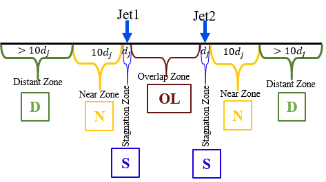
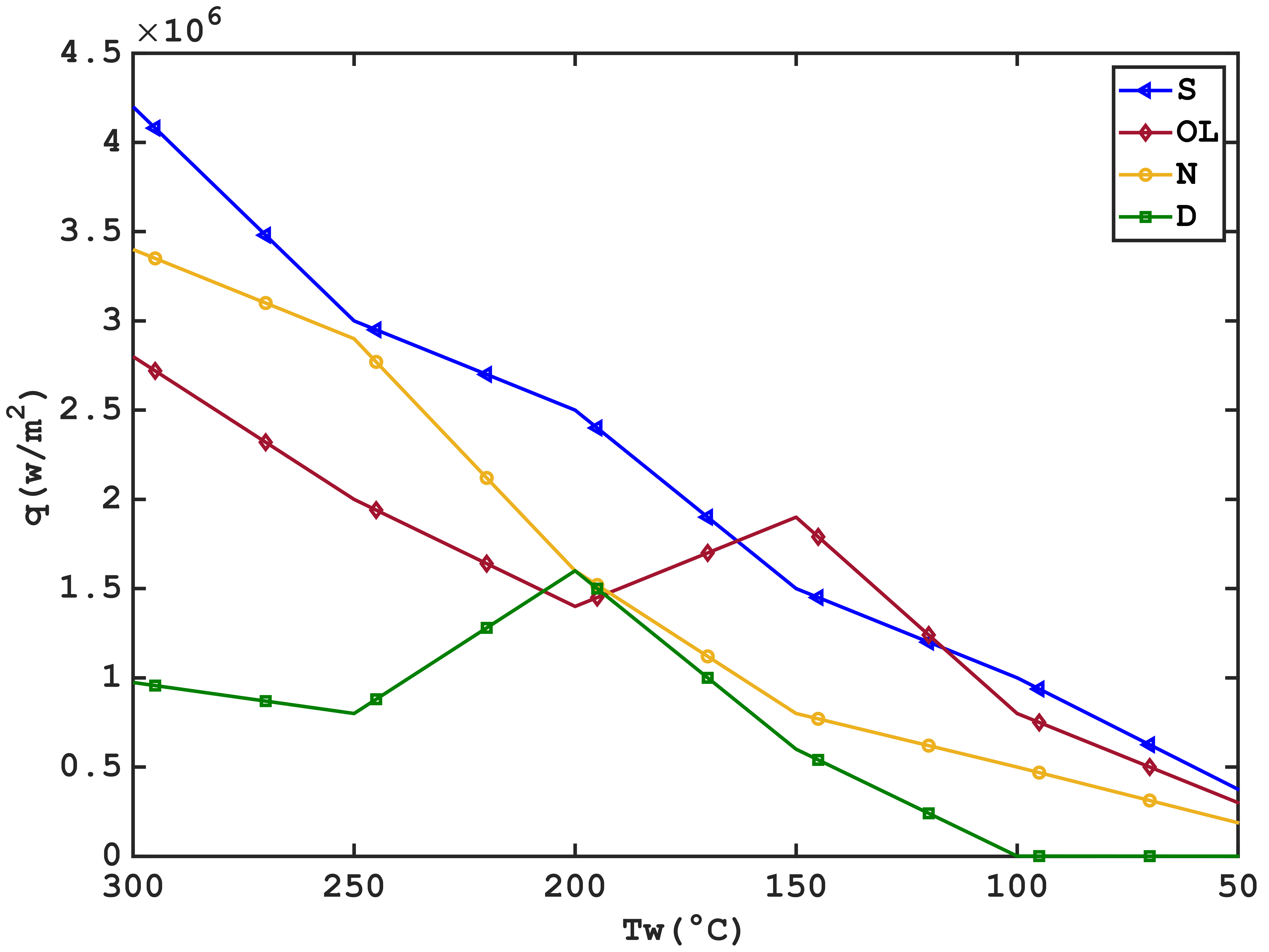
These values have been interpolated to construct the curves of the zonal variation of heat flux density, as shown in Figure 5.

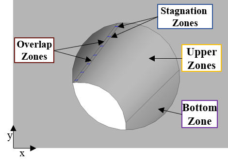
The projection of these results onto the current study is possible but requires the elimination of distant zones. Unlike the stagnation and overlap zones, which maintain similar characteristics, the other zones are significantly influenced by gravity and airflow. This contrasts with the plate scenario where water slides from the stagnation and heating zones to the rest of the plate, resulting in the delineation of four distinct cooling zones, as depicted in Figure 6.

The numerical model used for quantifying heat transfer on the wall is illustrated in the diagram in Figure 7.

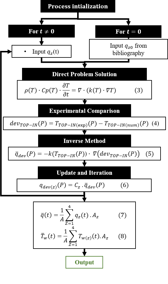
The process begins by imposing the initial values of the heat flux density for each zone q_z0 taken from the bibliography [15,27] for t=0 s as boundary inlet conditions.

The model then solves the direct problem using the heat transfer equation (Eq.3 in Figure 7), where ρ(T) is the density as a function of temperature, Cp(T) is the heat capacity as a function of temperature, and k(T) is the thermal conductivity as a function of temperature. This equation calculates the wall temperatures and temperatures at thermocouple locations.

Subsequent iterations involve comparing obtained values with experimental measurements (Eq.4 in Figure 7), where the deviation dev_TOP-IN(P) represents the difference between the experimentally measured temperature in TOP-IN points and the numerical values for all future time steps from 1 to 𝑃.

The inverse method is then used (Eq. 5 in Figure 7) to determine the average heat flux deviation for all future time steps from 1 to 𝑃.

Boundary conditions for each zone are adjusted using Eq. 6 in Figure 7, determining the heat flux density deviation for each zone q_dev(z)(P) for all future time steps from 1 to 𝑃 , using C_z the zonal area ratio calculated by Eq. 9

(9)

where A_z is the area of each zone and 𝐴 is the total wall area of 9.1 × 10^-2m^-2,

The model is updated and iterated by calculating average values over the four zones: the average heat flux (Eq. 7) and the average wall temperature (Eq. 8). These steps refine the model through an iterative process facilitated by MATLAB© and COMSOL© integration.

Preliminary work has been conducted to assess the impact of method parameters, without flow regulation, on the accuracy of the model. It revealed a degradation in accuracy when the time step exceeded 4 seconds or when the number of future time steps exceeded 5. Optimal precision is ensured by carefully selecting ideal values for calculations, with a time step (𝑑𝑡) of 4 s and a number of future time steps (𝑃) equal to 5.

Figure 8 represents the zonal values of thermal flux densities (q_z).

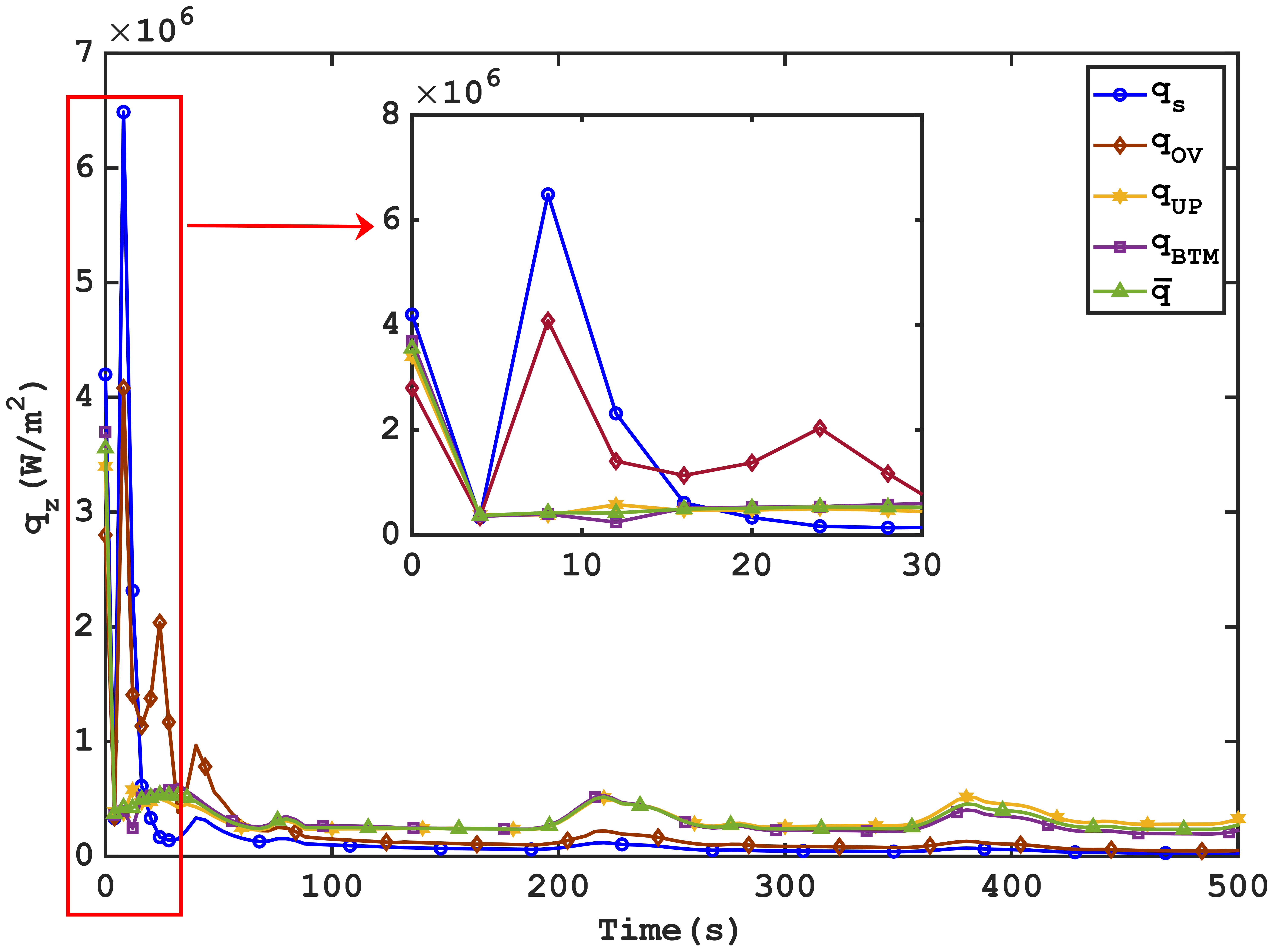
The analysis of zonal thermal flux densities (q_z) reveals concentrated thermal exchanges in the initial stages (20s), primarily in stagnation zones and jet overlap zones, where the thermal flux density values reach a maximum of 6.48 MW⋅ m^-2 and a 4.08 MW⋅ m^-2 respectively, while remaining below 0.62 MW⋅ m^-2 in the other two zones . The low average values observed are attributed to the extensive influence areas of the Upper and Bottom zones, which collectively represent over 98% of the total surface area of the cylindrical channel.

In the context of this parametric study, and in order to enable the evaluation of the influence of each parameter, the comparisons that follow in the subsequent sections is based on the variation of the average values of the heat flux densities applied to the wall as well as on the average wall temperatures over the entire wall calculated by Eq. 7 and 8 in Figure 7 .

3. 5. Numerical model results accuracy

In the validation of the numerical method, the deviation (dev_TOP-IN) from Eq. 4 in Figure 7 is first assessed by comparing numerical measurements to experimental values at the TOP-IN positions (in green in Figure 3). This parameter serves as a reference for the model's accuracy at these specific points. The numerical values at the TOP-IN positions are used to calibrate the thermal flux, which is then applied to the Near-Wall points (in yellow in Figure 3) to validate the model further. The calibration process involves adjusting the numerical model to minimize the discrepancy between the measured and simulated thermal fluxes at the TOP-IN points, ensuring the model accurately reflects the thermal behaviour observed experimentally using TOP-IN measurements for thermal flux calibration.

Figure 9 illustrates the comparison between numerical and experimental values

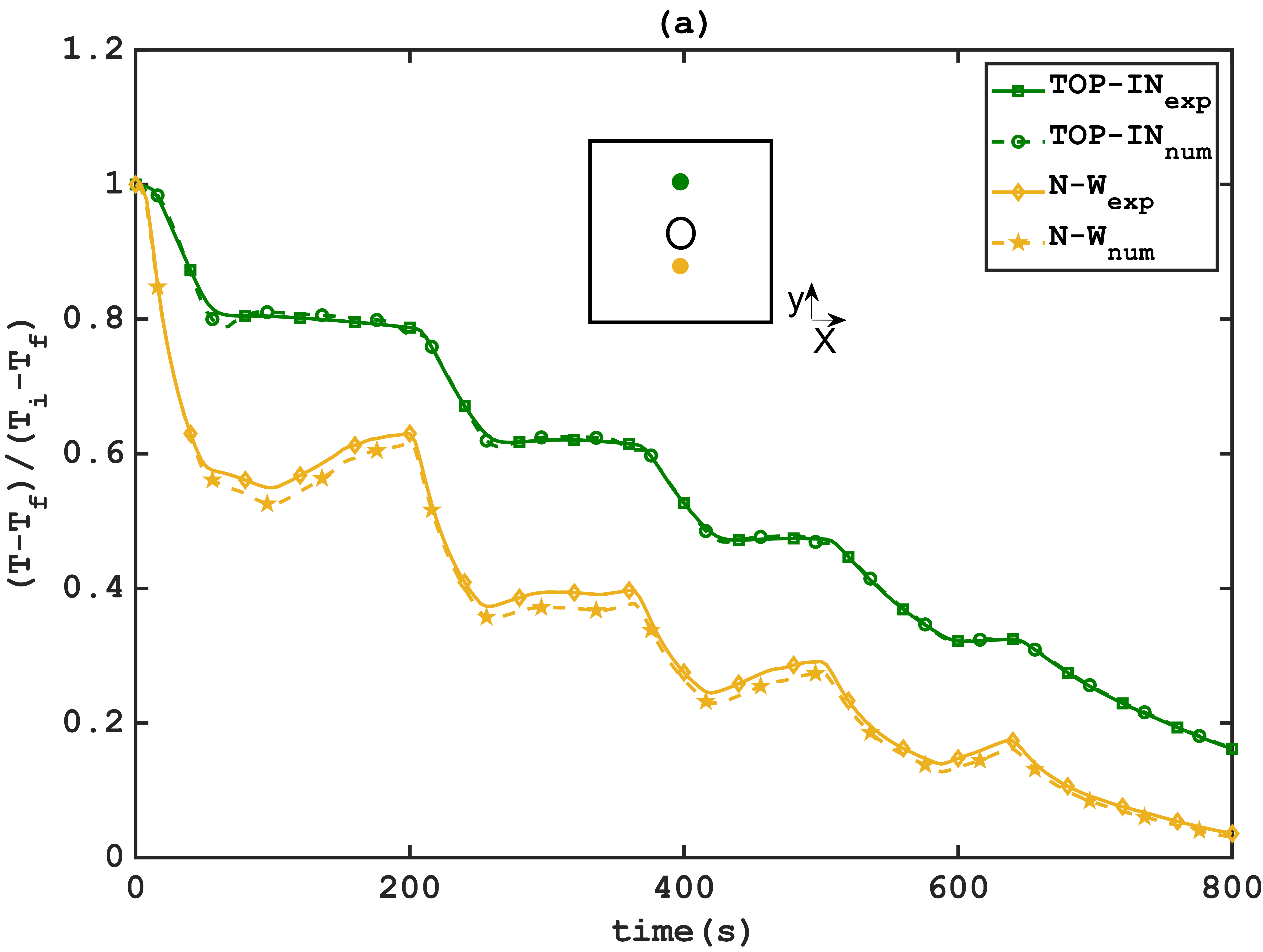
(a) Normalized variation
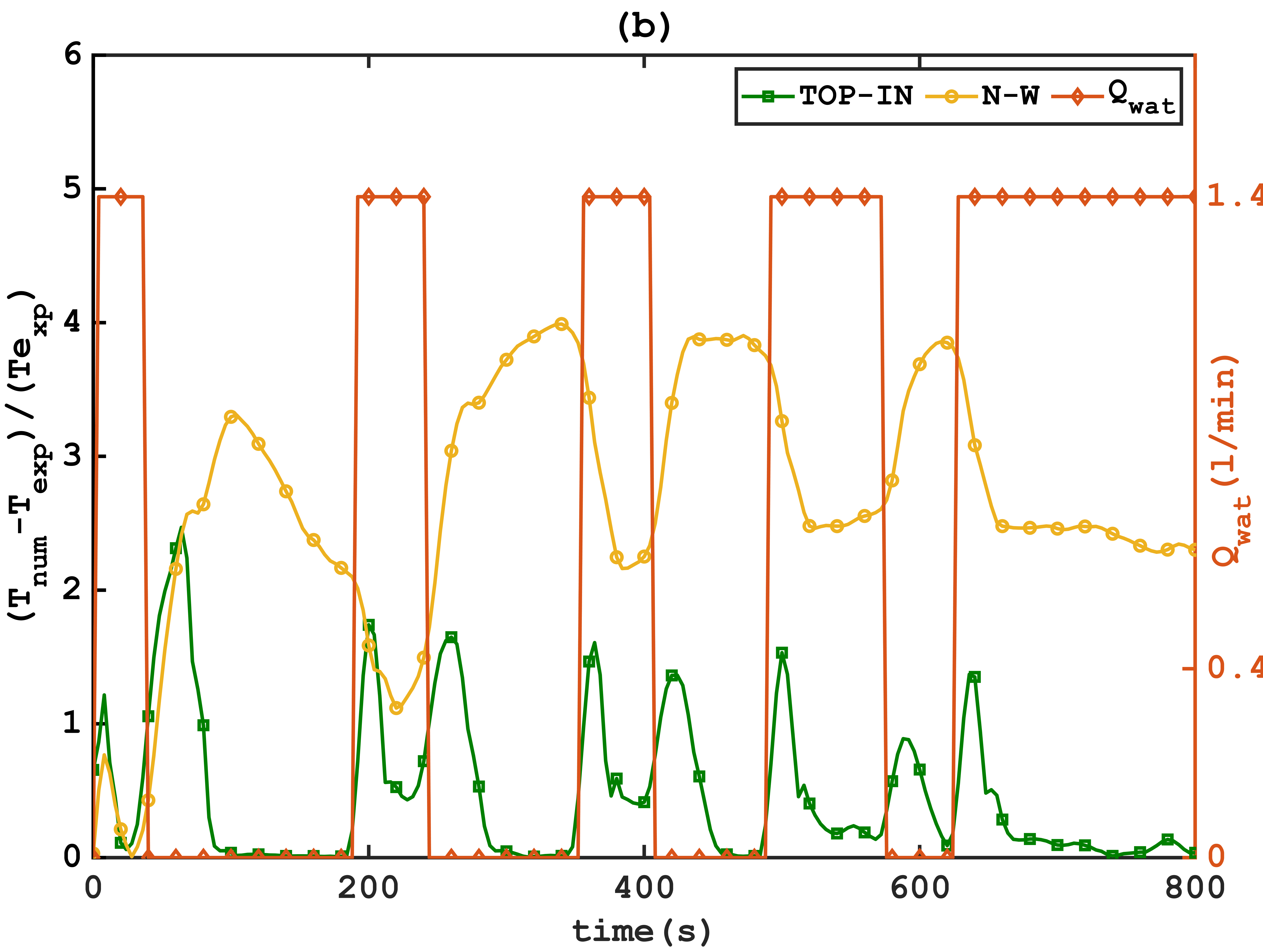
(b) Percentage error

Figure 9 reveals that the numerical and experimental values at the TOP-IN points closely match, with a relative error below 2.5%. This correlation indicates the model's robustness in predicting temperatures at these locations, attributed to the effective calibration process using TOP-IN measurements. However, when comparing the Near-Wall points, the errors are slightly higher due to the increased distance from the calibration points. The relative error at these points remains under 4%, which, while slightly higher, still demonstrates a reasonable level of accuracy given the complexity of the thermal phenomena being modelled. The model accurately predicts temperatures with a a Mean Squared Error (MSE) of 1.6 °C for TOP-IN points and 3.66 °C for Near-Wall points, validating the model's overall reliability and precision in capturing the complex thermal dynamics.

4. Results and discussion

4. 1. Reference case description

Figure 10 presents a reference with a water flow rate of Q_wat=1.4 l/min and an air flow rate of Q_a=40l/min.

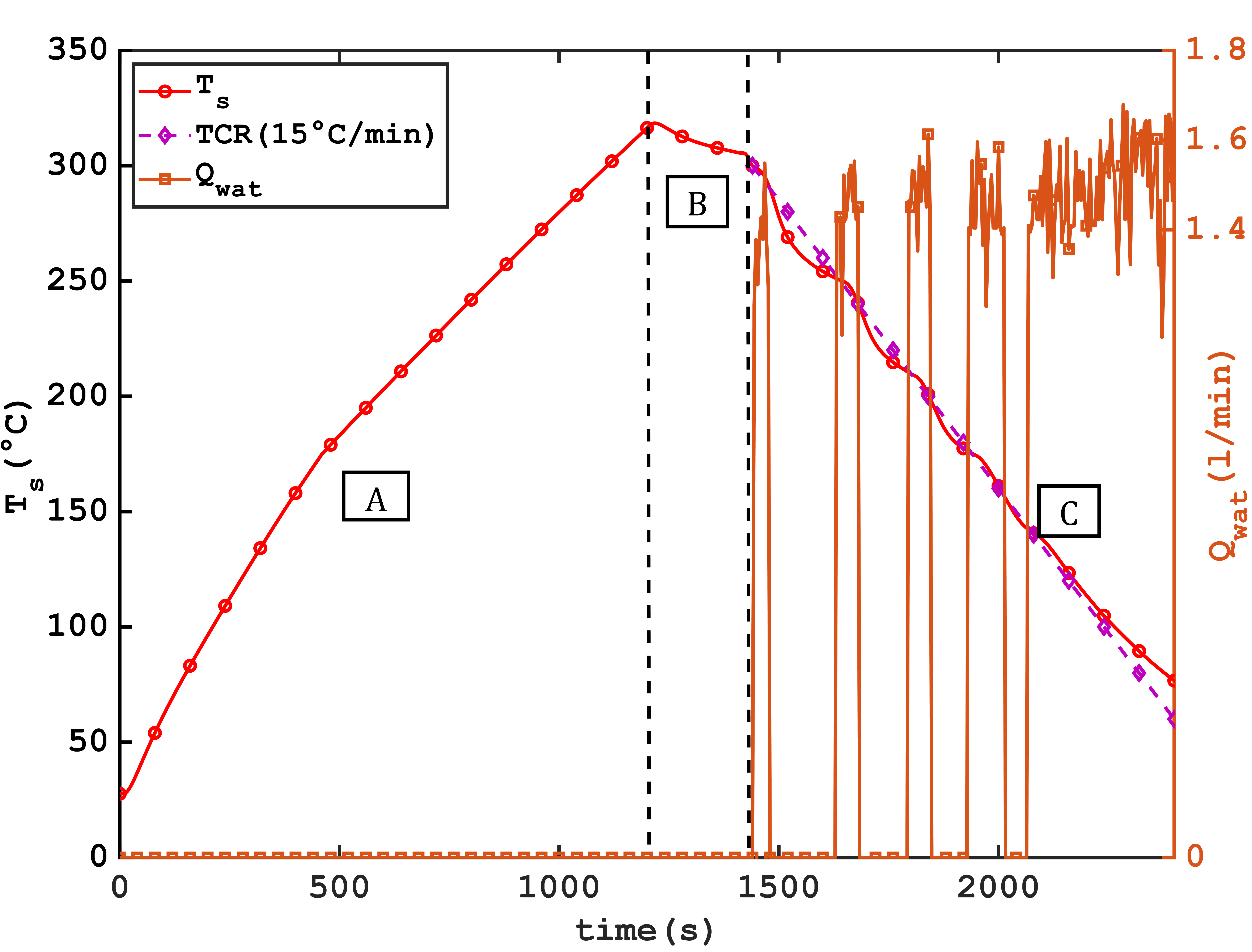
In Figure 10, the different operating cycles of the system are presented:

(A) Initial Heating at Low Airflow: The cycle starts with a heating phase until reaching 320 °C with an air flow of 14 "L/min" and a Reynolds number (Re_a) of 2000.

(B) Air Forced Cooling: Air cooling is employed to reduce the temperature from 320 °C to 300 °C, promoting temperature homogeneity on the upper surface. Natural convection also contributes to this process, albeit its impact is limited due to insulation presence.

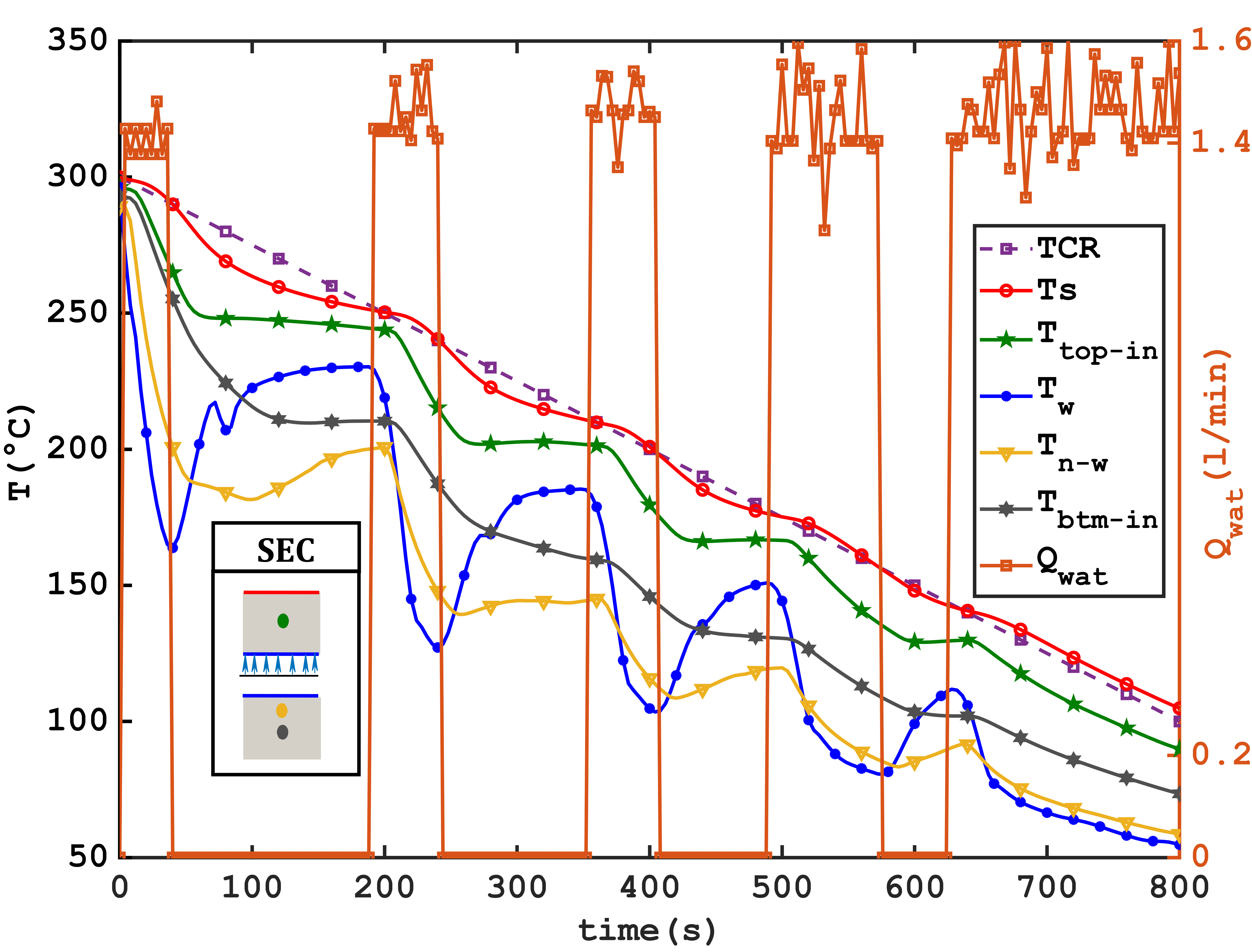
(C) Activation of Active Cooling: Active cooling is initiated once the average upper surface temperature reaches 300 °C, activating water jets and transverse airflow. Phase (C) is detailed in Figure 11, depicting cooling at different locations.

The numerical results obtained using the inverse method are represented by the blue curve.

The activation of water jets occurs as soon as the temperature of the block's upper surface (Ts) exceeds the setpoint temperature TCR. The response time, synchronized with the activation of the jets, shows an immediate response from the wall temperature calculated by the numerical model, with cooling rates reaching 356°C/min during the first cooling step. This rate gradually decreases in subsequent steps, dropping to 267°C/min for the second step and 109°C/min for the fifth step, likely due to the decrease in wall temperature and heat flux density exchanged with the wall. Variations in response time are observed: 10 s for thermocouples close to the wall (𝑇_𝑁−𝑊), 14 to 18 s for thermocouples located 15mm from the wall (𝑇_{𝑇𝑂𝑃−𝐼𝑁}) in green and (𝑇_{𝐵𝑇𝑀−𝐼𝑁}) in gray, and 28 s for thermocouples on the upper surface located 30 mm from the surface impacted by the jets.

Figure 11 clearly illustrates the effectiveness of the regulation algorithm in adhering to the prescribed cooling rate (TCR) of 15°C/min.

To explain variations in the average heat flux density exchanged with the wall during regulated cooling, experiments without regulation were conducted using the same air and water flow rates as presented in Figure 12.

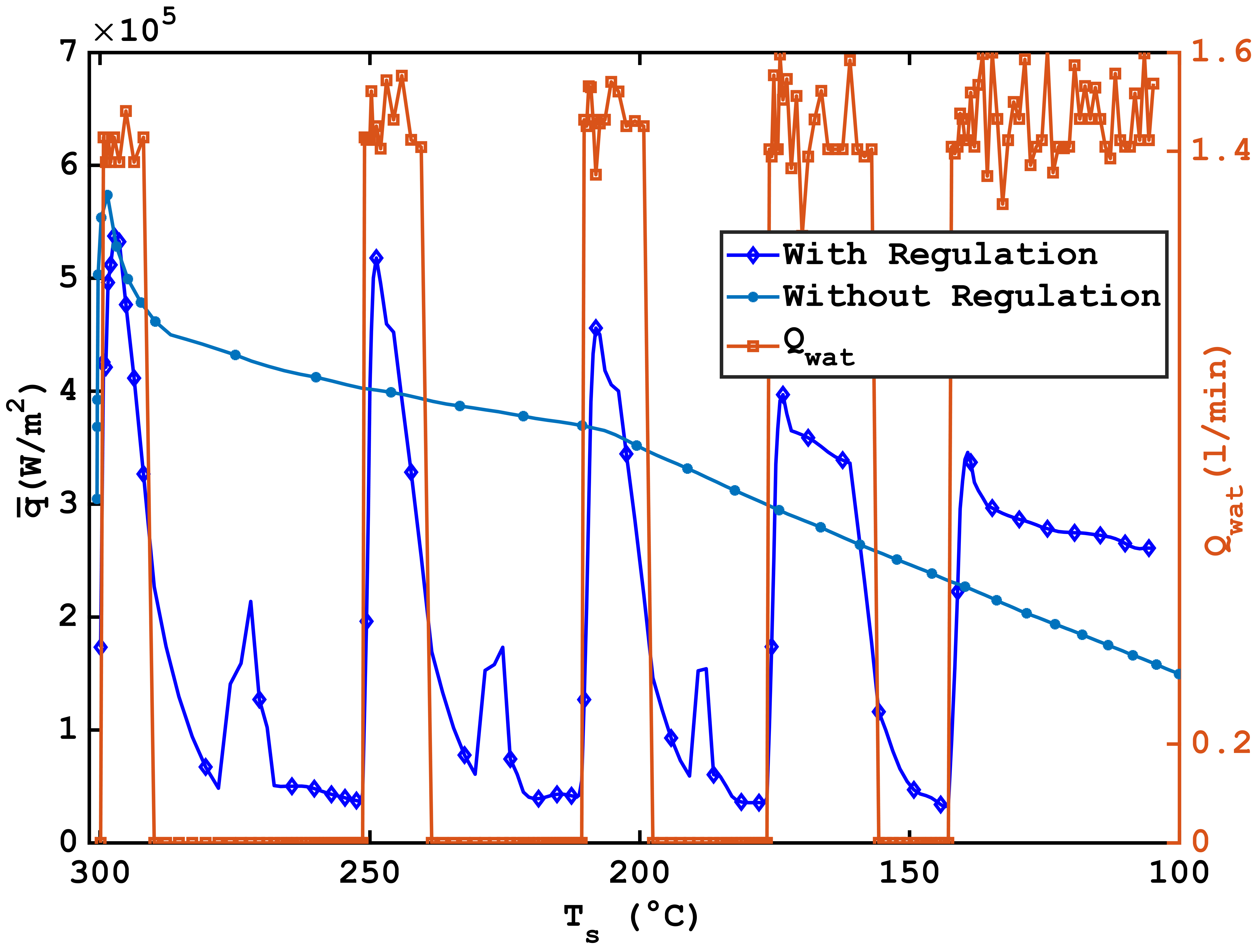
At the first step, a similar behavior is observed before where a maximum value of 5.73 × 10⁵ W/m2 is reached without regulation and a maximum of 5.28 × 10⁵ W/m² with jets stopped by the regulation algorithm to limit overshoot relative to the imposed cooling rate. However, discontinuous cooling generates higher heat flux densities upon jet restart, ranging from 5.17 × 10⁵ W/m² at the second step to 3. 45 × 10⁵ W/m²at the fifth step, compared to a decrease from 3.19 × 10⁵ W/m² to 1.29 × 10⁵ W/m²for unregulated cooling in the same temperature range. Peaks in heat flux density occur in the absence of jet activation, with values not exceeding 2.13 × 10⁵ W/m², representing 34 % of the main peak. This behavior on the wall after water flow cessation might results from cooling caused by water vapor resulting from the boiling of remaining water droplets in the cylindrical channel, leading to recondensation.

4. 2. Influence of flow ratio and jet orientation

In order to investigate the effect of jet flow ratios, two flow configurations with different mass flow rate ratios are employed. Additionally, to assess the influence of jet orientation, configurations with jets oriented downward, following gravity (180°), were utilized, contrasting the reference case where the jets are directed against gravity (0°). Table 1 summarizes the values of flow rates, mass flow rate ratios, and Reynolds numbers used in the experiments.

Table 1. Experimental parameters

N°	Tube	Qwat (l/min)	Rej	Qa (l/min)	Rea
1	7 j	1,4	4250	40	3500	4
2				350	30000	0,5
3	4J 1mm		7400	40	3500	7,3
4	4J 2mm		3700
5	19J 1mm		1550			1,5
6	19J 2mm		780

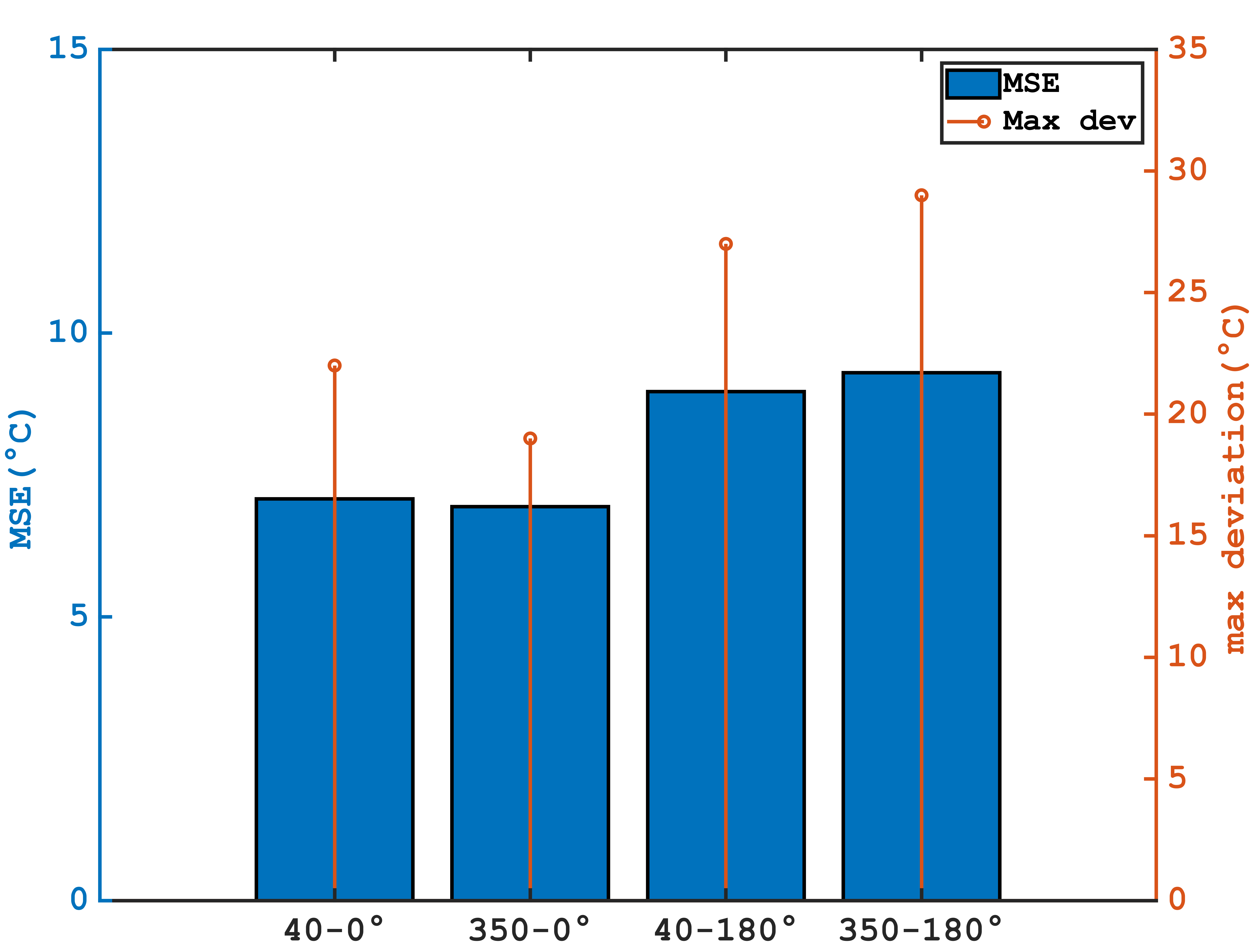
The cooling curves of the upper surfaces (Figure 13) and the corresponding deviations from the Target Cooling Rate (TCR) (Figure 14) demonstrate that reducing the mass flow rate ratio improves rate tracking, with a mean squared error (MSE) of 6.5 °C over the cooling period [0-800s] and a maximum deviation of 19 °C, compared to an MSE of 7.1°C and a maximum deviation of 22°C.

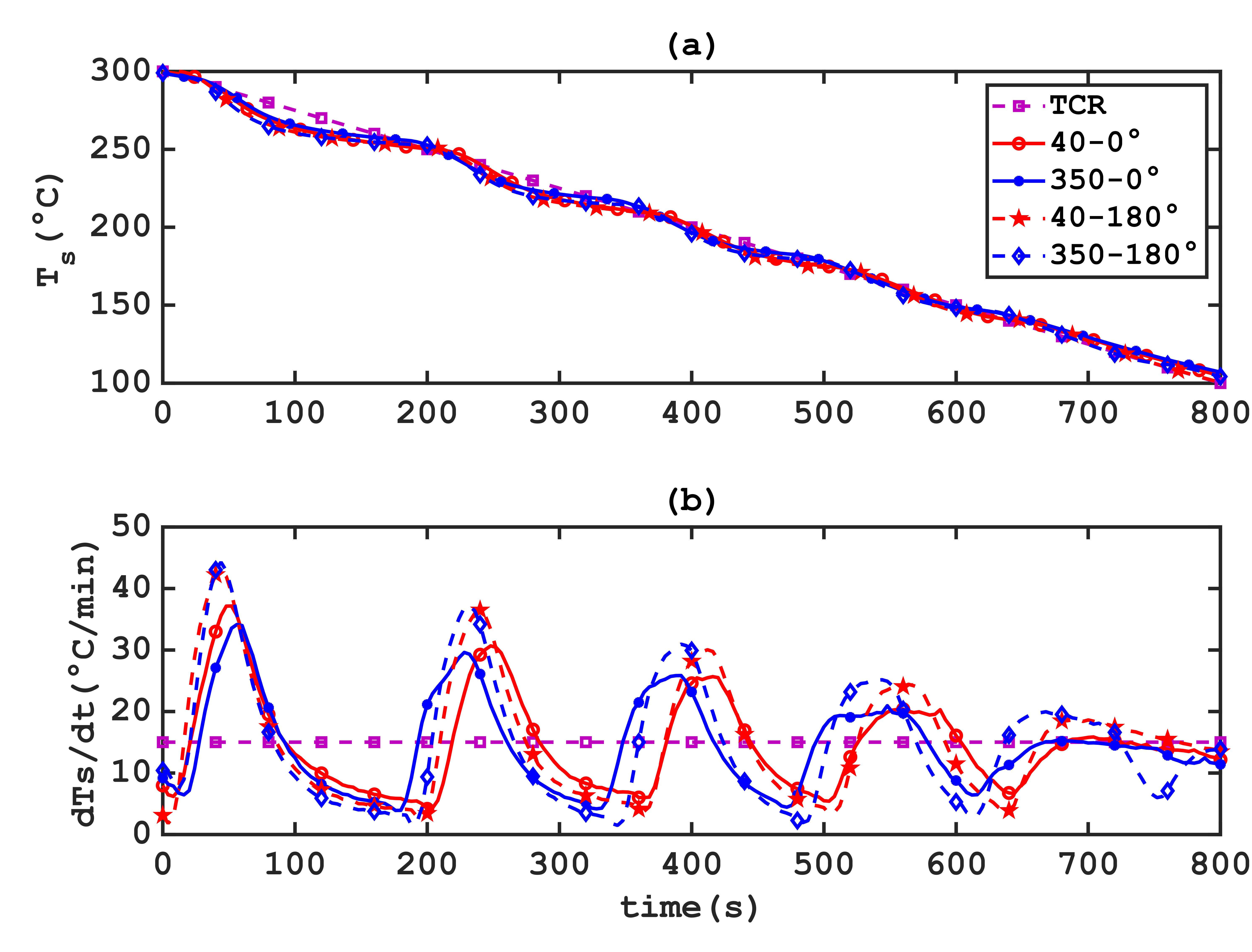
However, orienting the jets downward, in the direction of gravity, significantly impairs rate tracking, with an MSE increasing from 6.5°C to 9.4°C for high airflows.

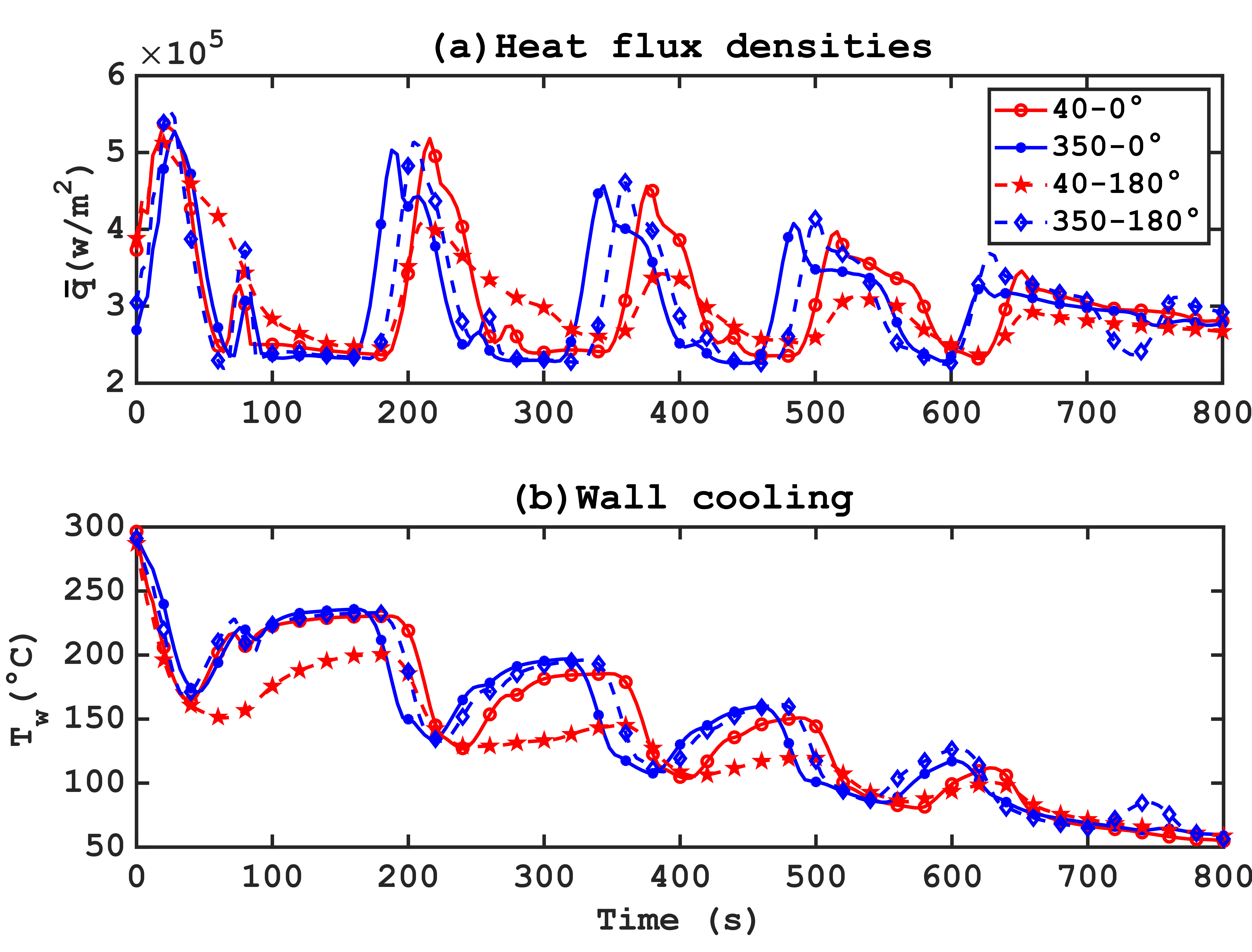
Regarding heat exchange at the wall level (Figure 15), the flow rate ratio has an almost negligible effect when flows are oriented against gravity. However, with low airflows and downward-oriented jets, a substantial deterioration in heat exchange is observed, attributable to the uneven distribution of the wetted area on the wall. When jets are oriented against gravity, the gravitational force efficiently removes water from the jets towards the outlet of the channel, promoting a uniform distribution of wall cooling and reducing residual vaporization. This hypothesis is supported by the absence of secondary peaks in the heat flux density curves during low airflow cooling oriented downward (dashed red curve in Figure 15).

To analyse the influence of Reynolds numbers and jet orientation on the uniformity of cooling on the upper surface in contact with the produced part, a two-dimensional assessment is conducted. Data from the 13 thermocouples aligned along the median line (represented in blue in Figure 2) are employed to assess uniformity along the length of the surface, while data from the 5 thermocouples located across the surface (denoted in orange in Figure 2) are used to evaluate uniformity across the width.

Considering the initial temperature difference at t=0, adjusted temperatures (X) are employed to eliminate this gap. The adjusted temperature expressed with Eq. (10).

(10)

is defined as the difference between the measured temperature T_i(t) at a given time and the temperature difference between this value and the average of temperatures T_i at t=0.

Next, to quantify variations in temperature in relation to the mean, providing insights into thermal fluctuations, the standard deviations SD are calculated using Eq. (11).

(11)

where i represents the thermocouple index (from 1 to 13 along the length and from 1 to 5 along the width) and n is the total number of considered thermocouples

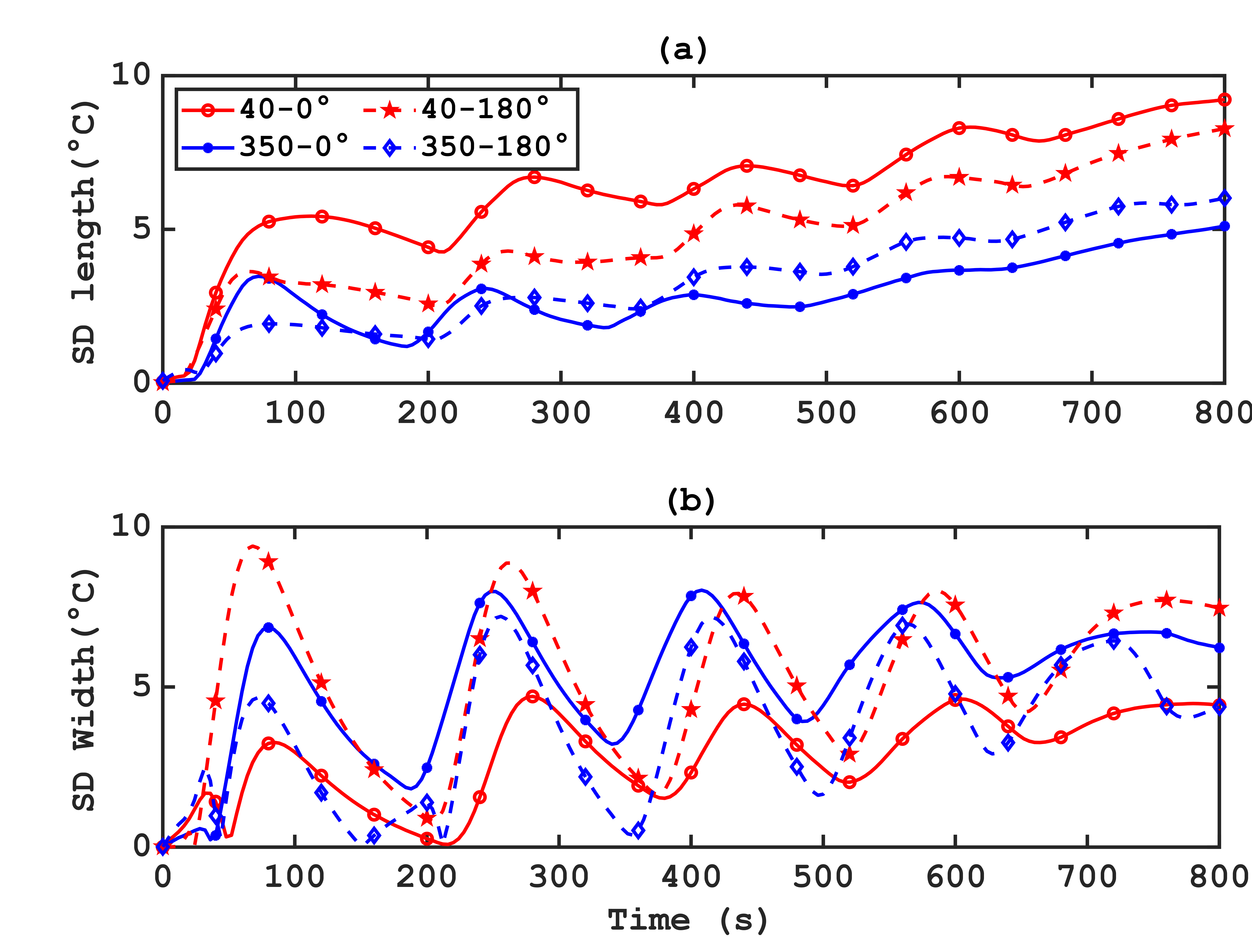
The results, varying with different ratios, are displayed in Figure 16. The analysis of this curves reveal that the uniformity of cooling varies depending on the cycles of jet activation and deactivation, facilitating heat transfer between hot and cold zones. A reduction in the mass flow rate ratio , along with increased airflow, improves uniformity along the upper surface, reducing the average standard deviation (which represents the mean value of the recorded standard deviations from 0 to 800 s) from 6.4 °C to 2.8 °C. However, across the width of the block, increases from 2.8°C to 5.2°C with increased airflow. The orientation of the jets in the direction of gravity (180°), with a reduced cooling rate, eliminates the effect of air ratio, reducing from 4.8 °C to 3.3 °C longitudinally and from 5.2 °C to 3.8 °C laterally.

4. 3. Influence of the size and distribution of water jets

To limit the influence of other parameters, the evaluation of jet diameter and number of jets is conducted using experiments 3-6 from Table 1, with a fixed water flow and air flow as in the reference case, and the jets oriented against gravity. When the diameter of the jets is increased to 2 mm, the D_h/d_j ratio becomes 3.75, and the jet spacing ratio D_j/d_j, will be 15. The influence of the number of jets and their diameters on the cooling of top surface is illustrated in Figure 17

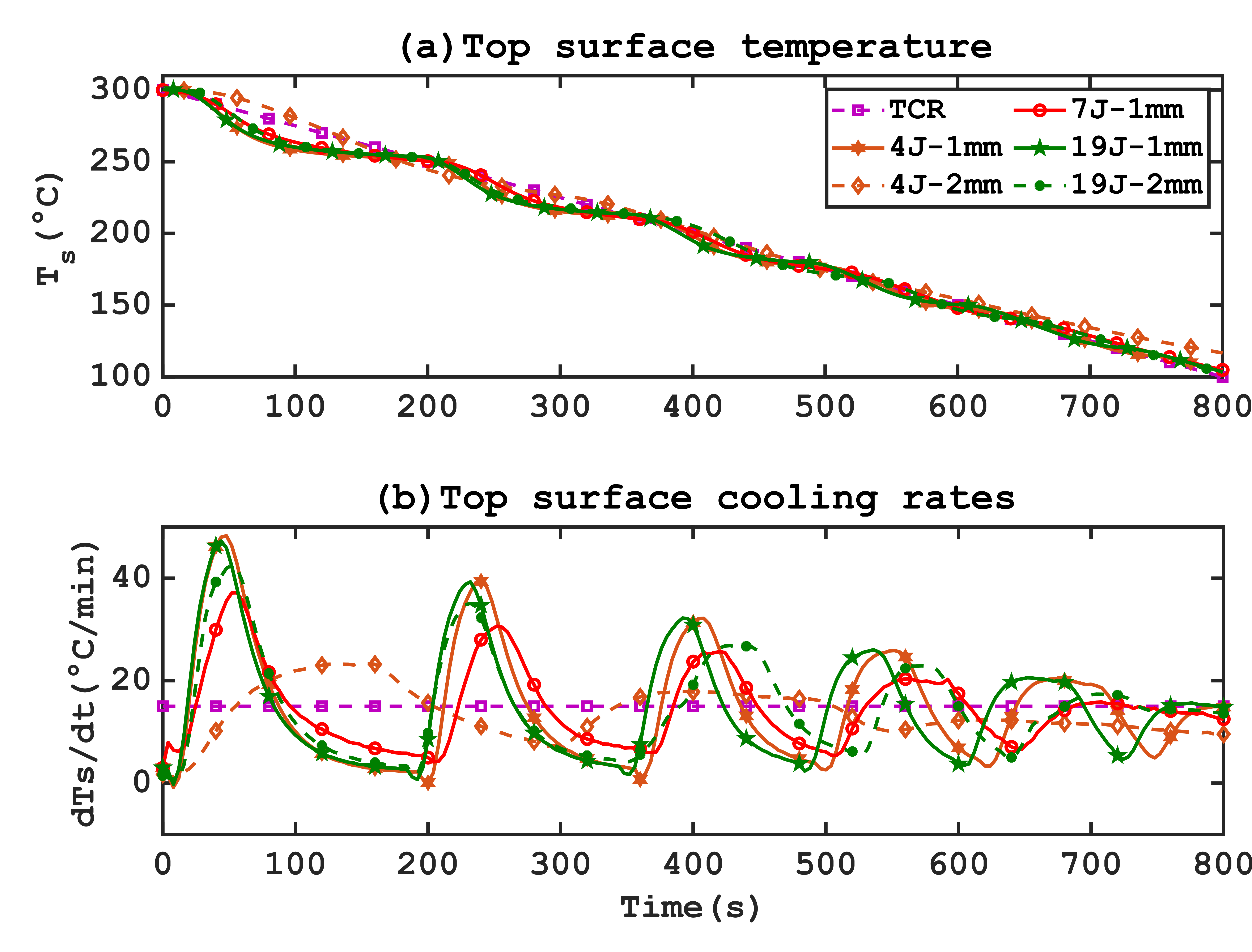
The analysis of these two parameters, presented in Figure 17, reveals that cooling with a tube of 7 jets significantly improves tracking of the setpoint as also shown in Figure 18 .

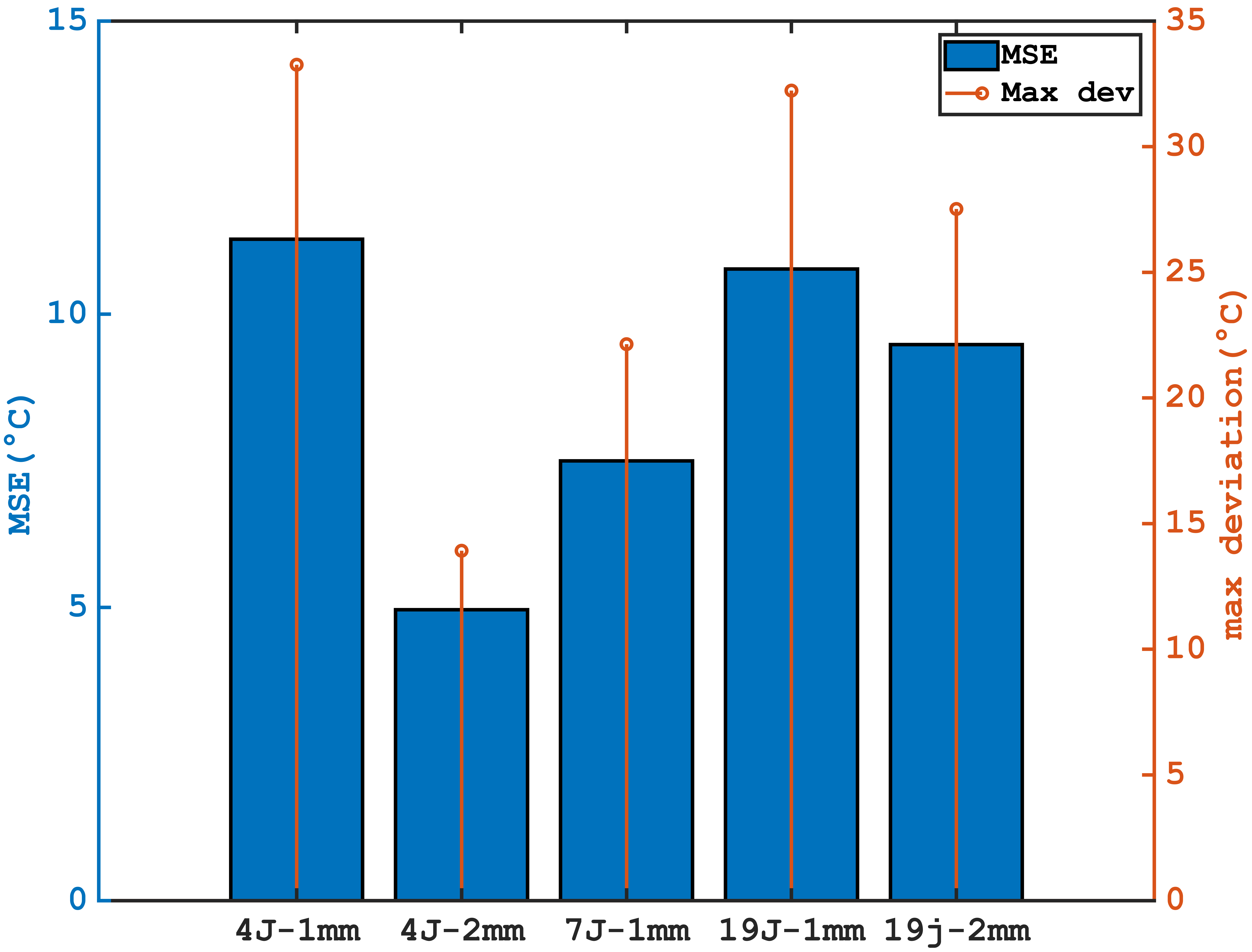
This observation aligns with previous experiments without cooling regulation and is consistent with literature [15], which emphasizes that an optimal number of jets allows for more effective cooling by avoiding excessive proximity or distance between the jets, promoting a more even distribution of wall cooling. This results in a reduction of the Mean Squared Error (MSE) from 11°C to 7°C and a reduction of the maximum deviation from 33°C to 20°C with an average number of jets. These conclusions also apply to heat exchange at the wall, where increasing the number of jets does not increase the intensity of heat exchange (Figure 19).

Regarding the effect of changing the diameter, which significantly affects jet velocity, it is observed on Figure 17 and Figure 18 that reducing jet velocity allows better tracking of the TCR, reducing the MSE from 11°C to 4.9°C for 4-jet tubes and from 9 °C to 4.9 °C for 19-jet tubes. This improvement is due to the slowed cooling resulting from reduced jet velocities. Given that the TCR is 15°C/min, using lower jet velocities is better suited to this type of cooling. However, if the imposed TCR exceeds 20°C/min, the effect is reversed, and the system can no longer follow the imposed TCR setpoint, as previously observed with unregulated flows.

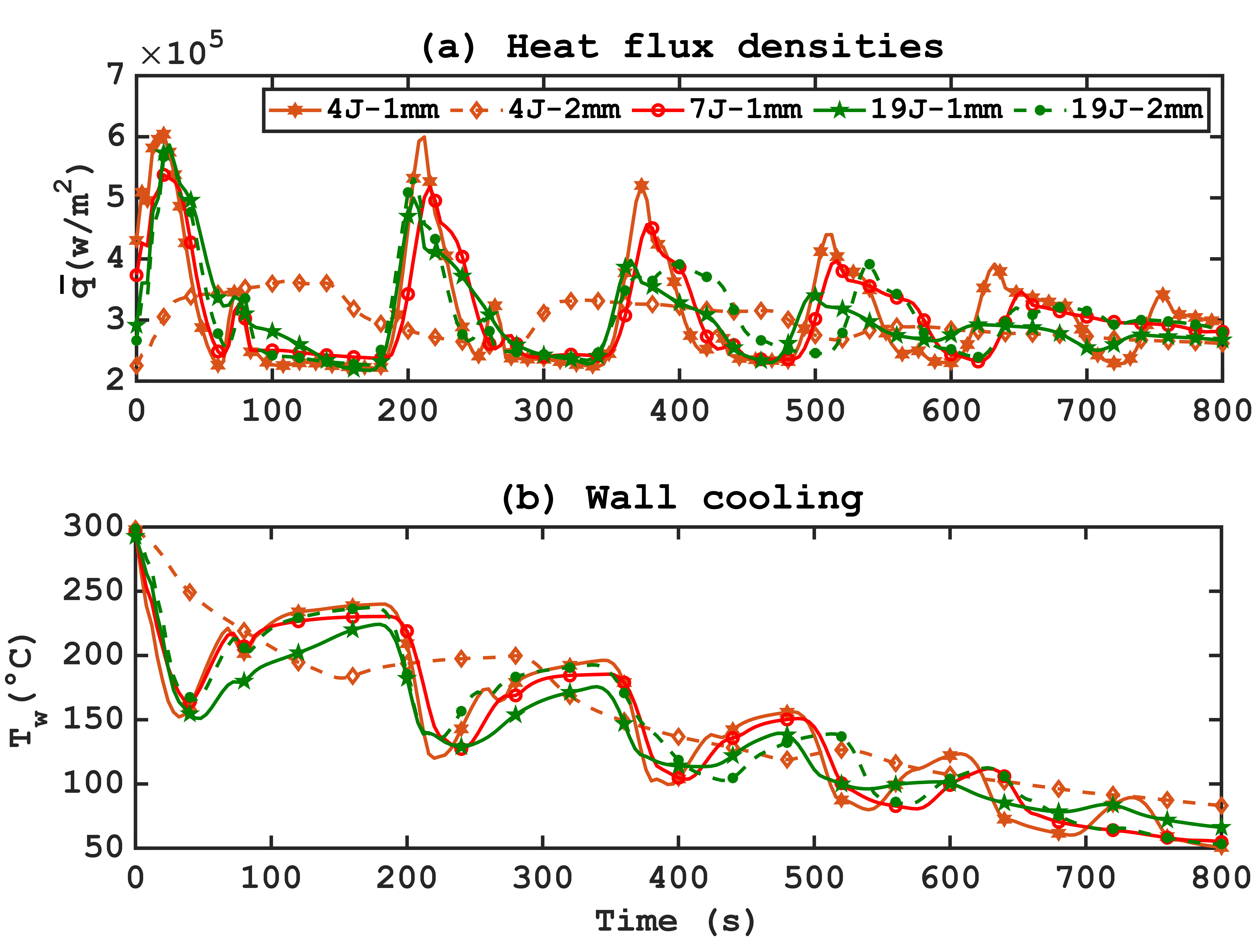
The heat exchange curves at the wall on Figure 19 confirm these observations, showing a significant loss of heat exchange intensity with larger diameters, decreasing from 482°C/min to 100°C/min for 4-jet tubes, with a less pronounced effect for 19-jet tubes, proportional to the difference in jet velocities.

Regarding uniformity in Figure 20, although the configuration with 7 jets improves uniformity along the length of the inner wall, this advantage is not observed on the upper surface.

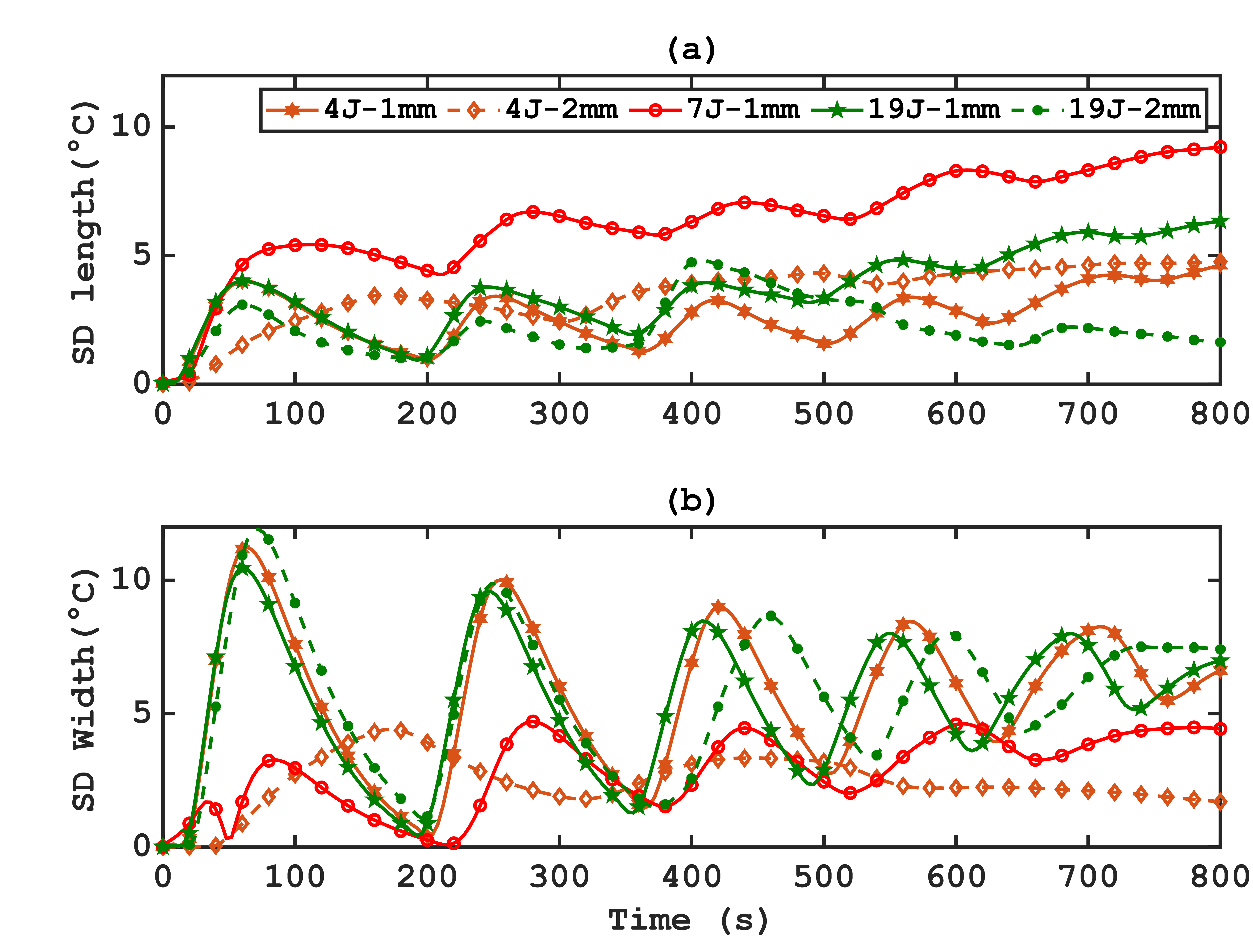
On the other hand, increasing the diameter reduces the cooling rate, improving homogeneity in width and on the upper surface decreases from 5.6°C to 2.4°C. The results suggest complexity in the relationship between flow parameters and cooling homogeneity. It should be noted that the shape of the curve for the 7-jet configuration in Figure 20 is primarily due to the position of the reference line in width, coinciding exactly with the central jet of the 7-jet configuration, allowing for better cooling of this line. However, this does not imply that this configuration results in superior uniformity in width on the upper surface, as the improvement of this criterion is directly related to the position of the jets and the cooling rate.

5. Conclusion

The comprehensive analysis of cooling mechanisms through impinging jets within the context of thermal regulation reveals several crucial findings. The meticulously calibrated experimental setup, characterized by different hydraulic and aerodynamic parameters, provides a solid foundation for the thorough analysis of heat exchange distribution in the impinging jet cooling system with transverse airflow. The numerical approach accurately quantifies heat transfers at the wall impacted by fluid flows, showing remarkable comparisons between experimental data and numerical results. The orientation of jets relative to gravity, the mass flow rate ratio , and jet diameter significantly influence cooling performance. Jets oriented against gravity favour even cooling distribution, while smaller jet diameters enable better low TCR tracking. Temperature uniformity on the upper surface of the test element is extensively evaluated, showing variations in uniformity depending on parameters, with longitudinal gains in uniformity and lateral losses, depending on jet orientation and flow rate ratio.

An optimal configuration, derived from this study, involves a tube with 7 jets spaced 30mm apart and a diameter of 1mm, oriented against the direction of gravity. This setup appears most suitable for imposed cooling rates between 10 and 20°C/min. However, this configuration requires adjustment if the imposed rate is lower or higher than this range to maintain optimal cooling performance.

In summary, this research contributes to a better understanding of impinging jet cooling mechanisms while identifying optimization opportunities to ensure efficient and uniform thermal management. These findings offer promising prospects for designing more effective cooling systems in various industrial applications, particularly in the field of thermoplastic matrix composite materials, where precise temperature control is essential for ensuring product quality. The ongoing commitment to addressing these cooling challenges will contribute to improvements in industrial manufacturing processes.

Acknowledgements

This project is funded by the IRT Jules Verne Technological Research Institute as part of their PERFORM program. We would like to extend our sincere gratitude to the SATER team at the GEPEA laboratory for their daily contributions to the commissioning and improvement of the experimental setup

References

[1] L. Yi, H. Hu, C. li, Y. Zhang, S. Yang, and M. Pan, 'Experimental investigation on enhanced flow and heat transfer performance of micro-jet impingement vapor chamber for high power electronics', International Journal of Thermal Sciences, vol. 173, p. 107380, Mar. 2022, doi: 10.1016/j.ijthermalsci.2021.107380. View Article
[2] R. D. Plant, J. Friedman, and M. Z. Saghir, 'A review of jet impingement cooling', International Journal of Thermofluids, vol. 17, p. 100312, Feb. 2023, doi: 10.1016/j.ijft.2023.100312. View Article
[3] T.-H. Wang and W.-B. Young, 'Study on residual stresses of thin-walled injection molding', European Polymer Journal, vol. 41, no. 10, pp. 2511-2517, Oct. 2005, doi: 10.1016/j.eurpolymj.2005.04.019. View Article
[4] A. Agazzi, V. Sobotka, R. LeGoff, and Y. Jarny, 'Optimal cooling design in injection moulding process - A new approach based on morphological surfaces', Applied Thermal Engineering, vol. 52, no. 1, pp. 170-178, Apr. 2013, doi: 10.1016/j.applthermaleng.2012.11.019. View Article
[5] Z.-C. Lin and M.-H. Chou, 'Design of the cooling channels in nonrectangular plastic flat injection mold', Journal of Manufacturing Systems, vol. 21, pp. 167-186, Dec. 2002, doi: 10.1016/S0278-6125(02)80160-1. View Article
[6] H.S. Park and X.P. Dang, Design and simulation-based optimization of cooling channels for plastic injection mold, New Technol.- Trends Innov. Res., PP.19-44, 2012 View Article
[7] X. Chen, Y. C. Lam, and D. Q. Li, 'Analysis of thermal residual stress in plastic injection molding', Journal of Materials Processing Technology, vol. 101, no. 1, pp. 275-280, Apr. 2000, doi: 10.1016/S0924-0136(00)00472-6. View Article
[8] H. Hassan, N. Regnier, C. Pujos, E. Arquis, and G. Defaye, 'Modeling the effect of cooling system on the shrinkage and temperature of the polymer by injection molding', Applied Thermal Engineering, vol. 30, no. 13, p. 1547, 2010. View Article
[9] O. Zoellner, 'Optimised mould temperature control', Applied Information Technology, vol. 1104, 1997.
[10] M. Balthazar, N. Baudin, J. Soto, D. Edelin, S. Guéroult, and V. Sobotka, 'Design of composite forming tool with high thermal dynamic through the use of lattice structures', in SAMPE Europe Conference 2023, Madrid, Spain, Oct. 2023. Accessed: Nov. 13, 2023. [Online]. Available: View Article
[11] C.-C. Kuo, Z.-F. Jiang, M.-X. Yang, B.-J. You, and W.-C. Zhong, 'Effects of cooling channel layout on the cooling performance of rapid injection mold', Int J Adv Manuf Technol, vol. 114, no. 9, pp. 2697-2710, Jun. 2021, doi: 10.1007/s00170-021-07033-2. View Article
[12] G. Wang, Y. Hui, L. Zhang, and G. Zhao, 'Research on temperature and pressure responses in the rapid mold heating and cooling method based on annular cooling channels and electric heating', International Journal of Heat and Mass Transfer, vol. 116, pp. 1192-1203, Jan. 2018, doi: 10.1016/j.ijheatmasstransfer.2015.09.126. View Article
[13] V. S. Devahdhanush and I. Mudawar, 'Review of Critical Heat Flux (CHF) in Jet Impingement Boiling', International Journal of Heat and Mass Transfer, vol. 169, p. 120893, Apr. 2021, doi: 10.1016/j.ijheatmasstransfer.2020.120893. View Article
[14] V. S. Devahdhanush and I. Mudawar, 'Critical Heat Flux of Confined Round Single Jet and Jet Array Impingement Boiling', International Journal of Heat and Mass Transfer, vol. 169, p. 120857, Apr. 2021, doi: 10.1016/j.ijheatmasstransfer.2020.120857. View Article
[15] S. G. Lee, M. Kaviany, and J. Lee, 'Quench subcooled-jet impingement boiling: Two interacting-jet enhancement', International Journal of Heat and Mass Transfer, vol. 126, pp. 1302-1314, Nov. 2018, doi: 10.1016/j.ijheatmasstransfer.2018.05.113. View Article
[16] R. Surya Prakash, A. Sinha, G. Tomar, and R. V. Ravikrishna, 'Liquid jet in crossflow - Effect of liquid entry conditions', Experimental Thermal and Fluid Science, vol. 93, pp. 45-56, May 2018, doi: 10.1016/j.expthermflusci.2015.12.012. View Article
[17] D. Thibault, M. Fenot, G. Lalizel, and E. Dorignac, 'Experimental study of heat transfer from impinging jet with upstream and downstream crossflow', presented at the turbine-09. Proceedings of International Symposium on Heat Transfer in Gas Turbine Systems, Begel House Inc., 2009. doi: 10.1615/ICHMT.2009.HeatTransf GasTurbSyst.490. View Article
[18] K. Yogi, S. Krishnan, and S. V. Prabhu, 'Local Heat Transfer of a Smooth Flat Plate Impinged by Multiple Jets', Heat Transfer Engineering, vol. 0, no. 0, pp. 1-18, 2024, doi: 10.1080/01457632.2024.2337975. View Article
[19] I. Piya, A. Kumar, N. Kaewchoothong, and C. Nuntadusit, 'Flow and heat transfer characteristics of submerged impinging air-water jets', International Journal of Thermal Sciences, vol. 193, p. 108503, Nov. 2023, doi: 10.1016/j.ijthermalsci.2023.108503. View Article
[20] G. Tymen et al., 'Temperature mapping in a two-phase water-steam horizontal flow', Experimental Heat Transfer, vol. 31, no. 4, pp. 317-333, Jul. 2018, doi: 10.1080/08916152.2015.1410505. View Article
[21] E. Agyeman, D. Edelin, and D. Lecointe, 'Experimental Study of the Effect of a Cross Airflow on the Dynamics and Heat Transfer Performance of Impinging Circular Water Jets on a Concave Surface', Heat Transfer Engineering, 2021, doi: 10.1080/01457632.2021.1887640. View Article
[22] E. Agyeman, P. Mousseau, A. Sarda, D. Edelin, and D. Lecointe, 'Homogeneous and automated cooling of a mould segment by multiple water jet impingement and a cross air flow', Journal of Thermal Science and Engineering Applications, 2021, doi: 10.1115/1.4050569. View Article
[23] Y. Yen Kee, Y. Asako, T. Lit Ken, and N. A. Che Sidik, 'Uncertainty of Temperature measured by Thermocouple', ARFMTS, vol. 68, no. 1, pp. 54-62, Mar. 2020, doi: 10.37934/arfmts.68.1.5462. View Article
[24] S. Twomey, 'The application of numerical filtering to the solution of integral equations encountered in indirect sensing measurements', Journal of the Franklin Institute, vol. 279, no. 2, pp. 95-109, Feb. 1965, doi: 10.1016/0016-0032(65)90209-7. View Article
[25] B. Heinrich and B. Hofmann, 'Inverse Heat Conduction. Ill-Posed Problems'. Journal of Applied Mathematics and Mechanics, vol. 67, no. 3, pp. 212-213, 1987, doi: 10.1002/zamm.19870670331. View Article
[26] C. S. Kim, 'Thermophysical properties of stainless steels', Argonne National Lab., Ill. (USA), ANL-75-55, Sep. 1975. doi: 10.2172/4152287. View Article
[27] N. Karwa, T. Gambaryan-Roisman, P. Stephan, and C. Tropea, 'Experimental investigation of circular free-surface jet impingement quenching: Transient hydrodynamics and heat transfer', Experimental Thermal and Fluid Science, vol. 35, no. 7, pp. 1435-1443, Oct. 2011, doi: 10.1016/j.expthermflusci.2011.05.011. View Article