Journal of Fluid Flow, Heat and Mass Transfer (JFFHMT)

ISSN: 2368-6111

1. Introduction: Linear Momentum Theory, Power Coefficient, and the Betz Limit

Linear momentum theory applied to the operation of horizontal axis wind turbines (HAWTs) dates back at least to Betz [1] and provides one of the most accessible bases for conceptualizing the function of such devices. Given that many thorough treatments of the topic exist in the literature [2]-[4] we give only the most salient features here.

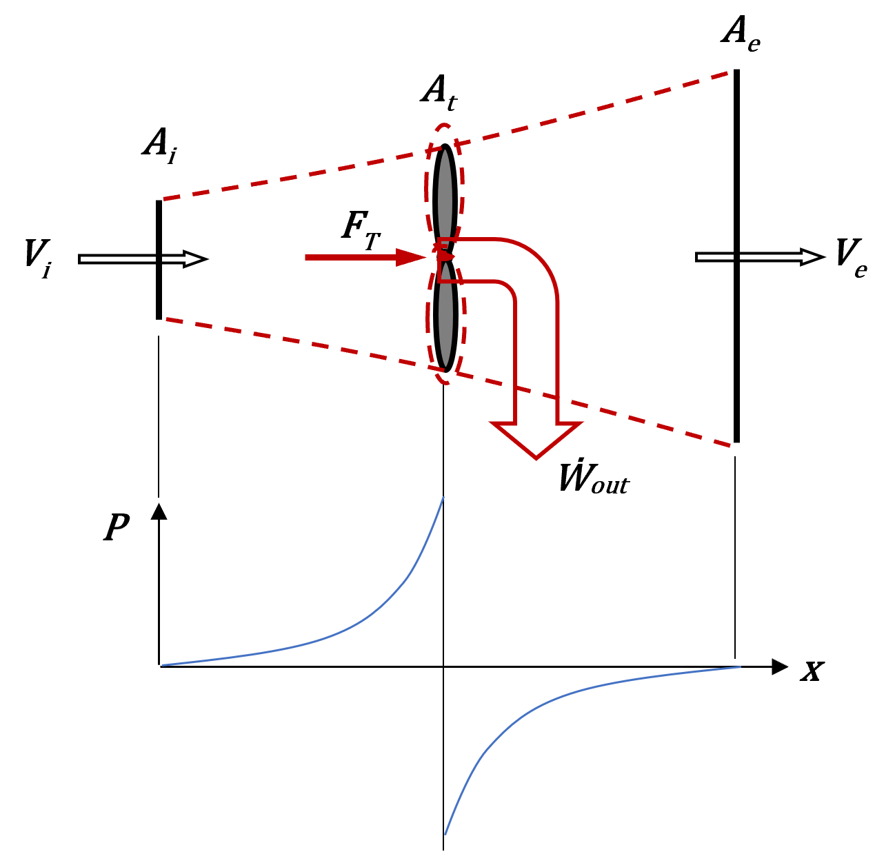
Figure 1 gives a side view of the analysed system, which consists of a diverging stream tube extending from the downstream side of the wind turbine to the upstream side. The variables V and A refer to wind speed and cross-sectional area, respectively, whereas F_T is the thrust force exerted on the hub by the wind and Ẇ_out is the power extracted by the turbine. The subscripts indicate the planes in which the windspeed corresponds to its undisturbed, freestream value (i), the value at the rotor plane (t), and the minimum downstream value before the wind reforms (e). Local static pressure varies in the flow direction but takes on atmospheric values at locations (i) and (e). The rotor sees a discontinuous drop in pressure in the flow direction and serves as the point at which all energy extraction occurs. With these idealizations the rotor is often referred to as an “actuator disc.” The flow is also modelled as incompressible with a density ρ, one-dimensional, isothermal, and frictionless.

Macroscopic mass, momentum, and energy balances applied to the system in Figure 1 result in a predicted value for developed power given by

where a is the axial induction factor, a parameter representing the fractional decrease in windspeed as the freestream wind approaches the actuator disc [2],

A common reference value for power in the operation of HAWTs is the “power in the wind,” the amount of kinetic energy per unit time in a flow of wind with a cross sectional area equivalent to the rotor swept area, A_t,

Expressing the developed power as compared to the power in the wind gives the traditional definition of power coefficient,

Equations 1, 3, and 4 are easily combined to show that linear momentum theory predicts power coefficient to be a function of axial induction factor only,

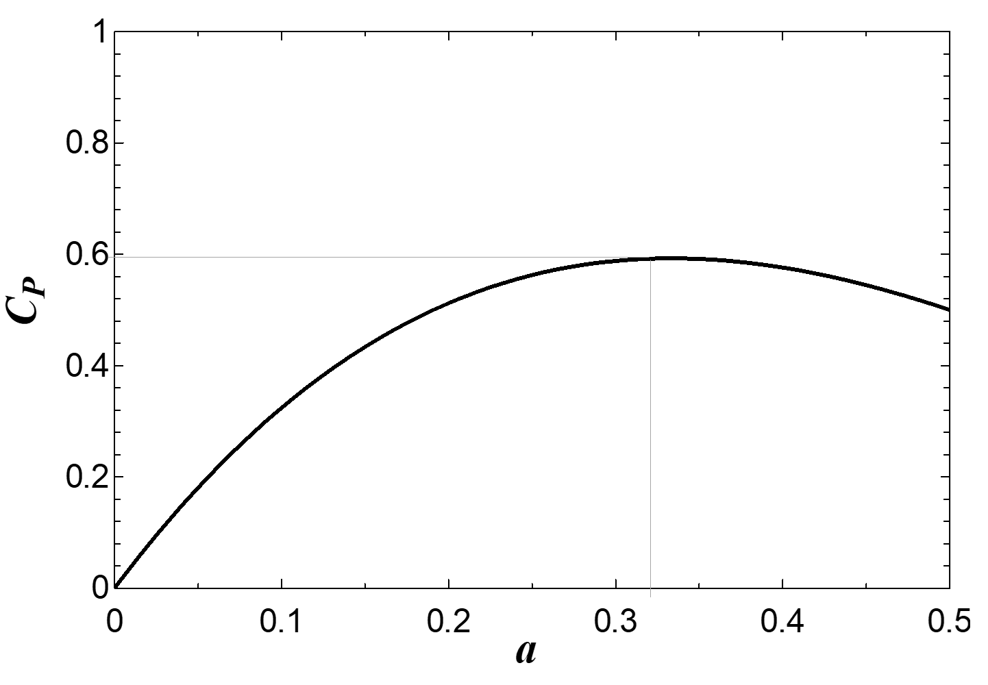
The polynomial form of Eq. 5 suggests a maximum value of C_P. Differentiating Eq. 5 with respect to axial induction factor and setting it equal to zero gives this maximum as 16/27, occurring at a value of a = 1/3 :

Equation (6) represents the famous Betz limit for wind turbine performance, stating that a HAWT can deliver a maximum of just under 60% (59.3%) of the “power in the wind.” Figure 2 shows the relationship of C_P to a based on linear momentum theory.

Linear momentum theory also gives a theoretical expression for the thrust the wind exerts on the actuator disc as

where C_T=4a(1-a) is the thrust coefficient. Unlike the power coefficient, the maximum value of thrust coefficient is C_T,max = 1, occurring at a = 1/2. Of note is that a = 1/2 corresponds to a wind speed of zero at (e) and that maximum power and maximum thrust are therefore not realised at the same value of axial induction factor.

We should also note that although linear momentum theory predicts power coefficient to be a function only of axial induction factor, the definitions of power in the wind and power coefficient given in Eqs. 3 and 4, respectively, are not subject to any of the assumptions of the theory. Indeed, the power coefficient of Eq. 4 is the most common measure of performance used for all real HAWTs with Eq. 5 often serving as an idealised upper limit used for purposes of comparison.

2. The Problem of Power Coefficient as Conversion Efficiency

Though the power coefficient likely serves as the most useful measure of performance for HAWTs, its interpretation as an energy conversion efficiency comes with several inconsistencies. Principal among these is what best represents the various inputs and outputs of energy. We outline the inconsistencies below.

2. 1. Competing Definitions of Efficiency

In defining a conversion efficiency, we typically track the input and output energy flows of a device, the efficiency being the ratio of the desired output to some input that represents the depletion of a resource. If the energy related quantities are power, then the efficiency becomes

where P_in is input power and P_out is the desired output power.

Implicit in employing such an efficiency is that part of the input power is not converted to the useful output, but rather to some other unusable form and/or that it is rejected elsewhere. Applied to the steady-state operation of a DC motor as in Figure 3, for example, only part of the input electrical power Ẇ_elec,in is converted to the desired mechanical power, Ẇ_out, the remaining input power being irreversibly dissipated as heat transfer to the surroundings, Q̇_out. This results in a conversion efficiency of η = Ẇ_out/Ẇ_elec,in.

If we consider the input to a wind turbine to be the power in the wind P_wind with a corresponding useful output of Ẇ_out, then Eq. 8 gives the efficiency to be

which is identical to the power coefficient of Eq. 4. Figure 2 above would therefore suggest that the efficiency of a HAWT can never be one, but rather can reach a maximum of only 16/27 at a = 1/3.

However, when considering the stream tube of Figure 1 from which the results of linear momentum theory are derived, we envision a different set of inputs/outputs. Figure 4 shows the system of Figure 1 from an energy perspective.

Conservation on energy as applied to the system of Figure 4 gives the power output as the difference between the inlet and exit kinetic energy flows:

where ṁ=ρA_iV_i is the mass flowrate of wind through the stream tube. Rearranging and making use of the axial induction factor,

The only energy input in Figure 4 is the flow of kinetic energy to the stream tube such that input power is P_in = ½ ρA_iV_i³. Thus the conversion efficiency of Eq. 8 becomes

Figure 5 gives a visualisation the conversion efficiency of Eq. 12.

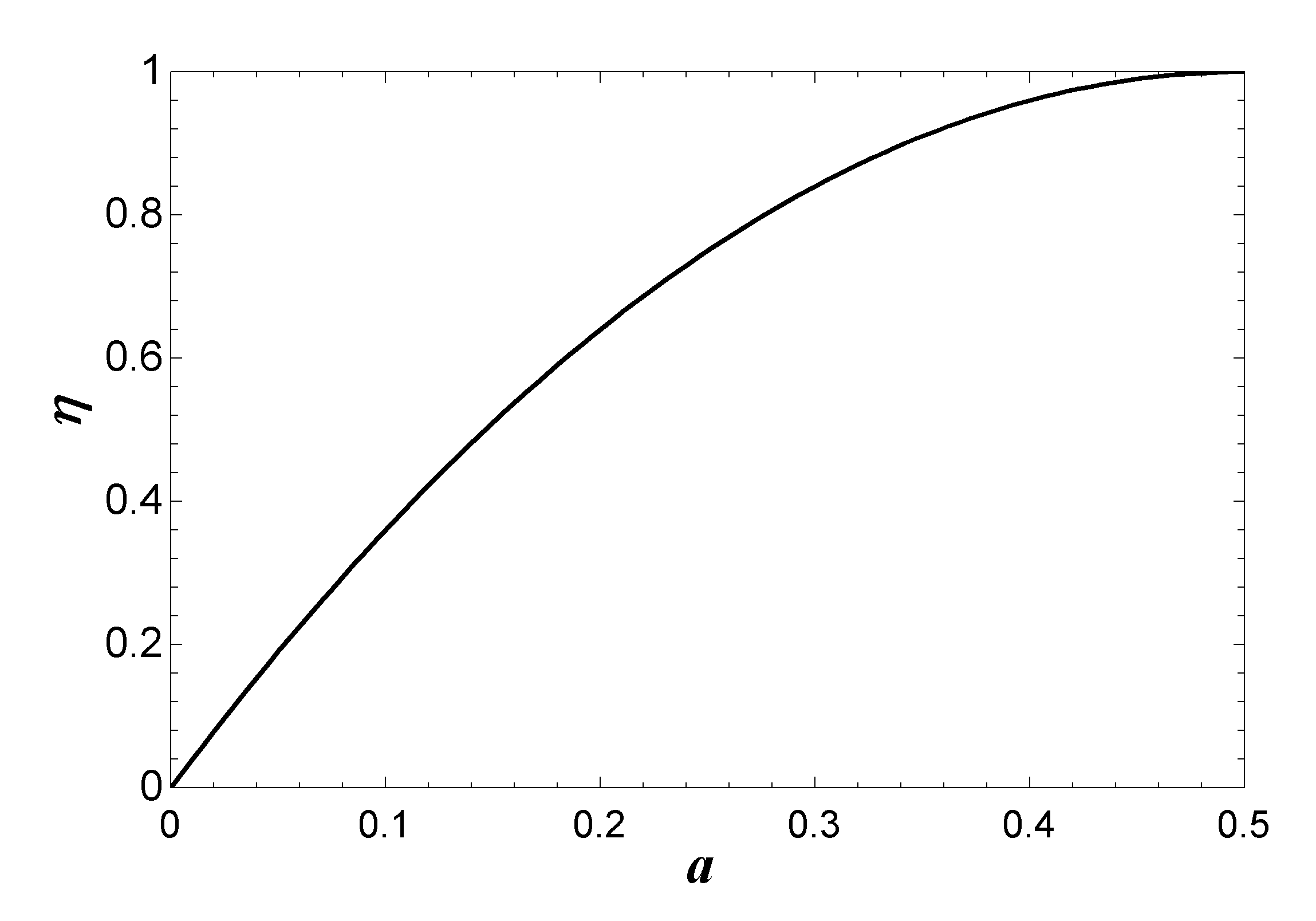
Clearly Figure 5 gives a much different picture of efficiency than Figure 2. Rather than a maximum value of 16/27, Figure 5 suggests that a HAWT can in fact achieve an efficiency of unity, and that that efficiency occurs at a=1/2, not at a=1/3. The reader may also recognize that the expressions for η and the thrust coefficient C_T (Eq. 7) are the same, implying that maximum efficiency and maximum thrust force are indeed achieved simultaneously, contrary to the common interpretation of power coefficient as an efficiency.

2. 2. Ambiguity of Inputs

The discrepancy between the two definitions for efficiency arises from the different assumed inputs for each. In Eq. 12, P_in corresponds to the power of the upstream wind for the actual mass flowrate passing through the actuator disc, ṁ = ρA_iV_i. On the other hand, P_wind is the power of a hypothetical mass flow of wind at speed V_i through the actuator area, A_t; that is, ṁ_wind = ρA_tV_i. In other words, P_wind is the power that would be contained in a cross-sectional area of A_t if the turbine were not present. As such some authors refer to P_wind as the “power of the undisturbed wind” [4].

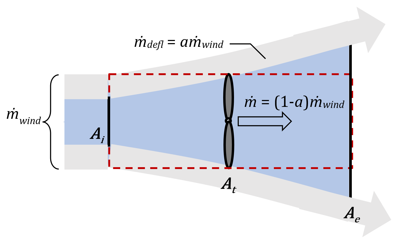
Figure 6 shows the air flow associated with the wind turbine and allows us to contrast the different flowrates. The blue shading corresponds to the actual mass flow through stream tube, ṁ=ρA_iV_i, whereas the grey shading is the mass flow associated with ṁ_wind that is diverted around the turbine, ṁ_defl. The mass flow corresponding to P_wind is the sum of the two, ṁ_wind = ṁ + ṁ_defl.

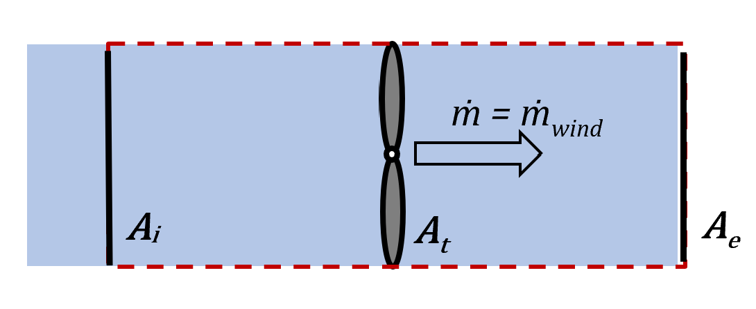
Since the speed of the flow decreases as it approaches the actuator disc, the incompressibility of the fluid requires that the upstream area A_i be less than that of the actuator disc, A_t. Consequently, the flow rate through the wind turbine ṁ must be less than ṁ_wind, becoming smaller still with increasing values of the axial induction factor. Tracking a quantity of ṁ_wind starting upstream of the actuator disc, we find that ṁ = (1-a)ṁ_wind makes its way through the actuator disc whereas ṁ_defl = aṁ_wind bypasses the actuator disc completely. Only in the case of zero power output, when a=0, does ṁ_wind = ṁ. (Fig. 6b.) We may therefore question whether P_wind truly represents the power input to the turbine, since it is the power associated with ṁ_wind and not with ṁ.

(a) (b)

Of the flow that does go through the actuator, a fraction η = 4a(1-a) of that is converted to mechanical power, the remainder exiting with the flow downstream through A_e. Hence, the power coefficient accounts for two different effects, the diversion of part of ṁ_wind around the actuator disc and the partial conversion of kinetic energy into power for the flow through the disc itself:

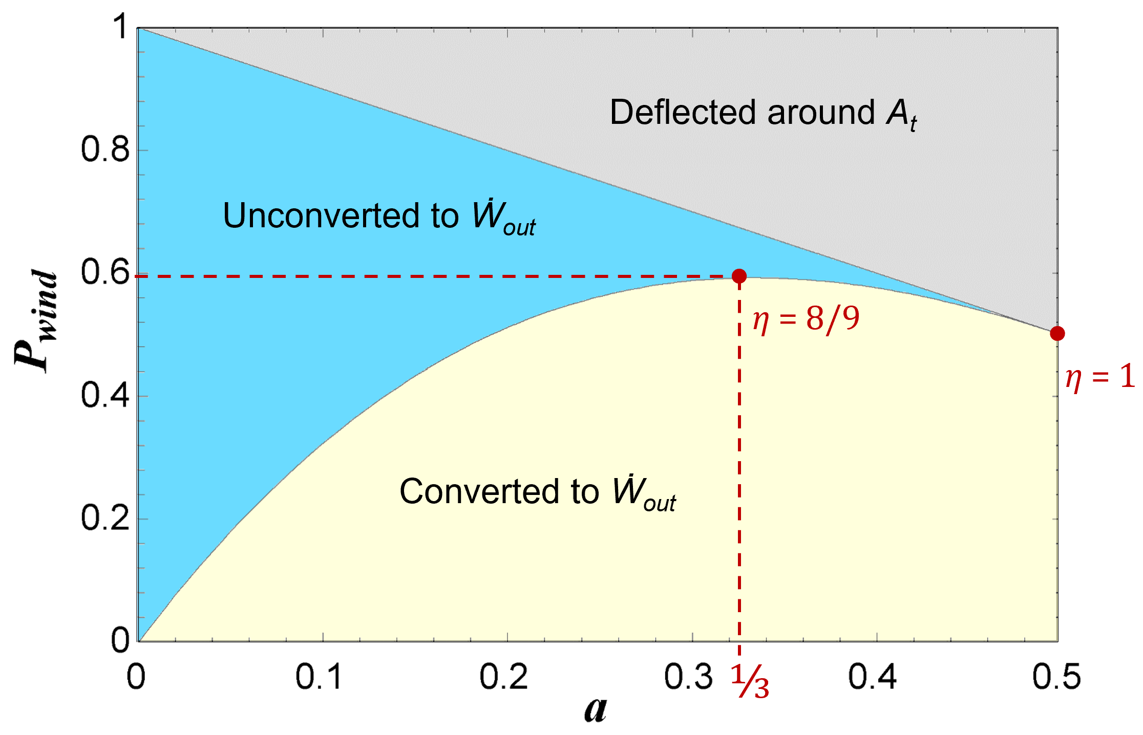
Figure 7 shows the relative proportions of P_wind as a function of axial induction factor. The figure gives additional insight into the power coefficient as shown in Figure 2 in that the two effects of Eq. 13 are distinguishable.

The maximum power output is realized at a =1/3 even though the conversion efficiency of Eq. 12 gives a value of η = 8/9 at that point. As a increases beyond 1/3, the power output decreases despite an increasing η due to smaller inputs of P_in delivered to the actuator disc. The trend continues until the total output of the turbine drops to 50% of P_wind at a=1/2 although η = 1.

(a)

3. Reinterpretation of Power Coefficient as a Measure of Performance

Resolving the ambiguity of C_P as an efficiency resides in its reinterpretation as a different measure of performance. Though we may loosely consider the power coefficient as an efficiency in that it compares power output to a conveniently calculable reference, with the result (usually) being less than unity, its interpretation as an energy conversion efficiency poses several difficulties. In particular, the discussion above demonstrates that such an interpretation of C_P would require us to make the rather awkward modelling assumption that a flow of wind travelling around the turbine—a flow that avoids the actuator disc altogether—constitutes part of the inputs and outputs of the device. Furthermore, linear momentum theory invokes isothermal and frictionless assumptions, which indicates reversible flow. Hence, there is no theoretical foundation from which to assert that 100% of the kinetic energy of a flow cannot be extracted as power. Indeed, this is what Eqs. 10 and 12 along with Figure 5 indicate, namely, that the rate of kinetic energy input P_in is completely converted to output power when the downstream area is very large and the speed V_e becomes vanishingly small.

And so, if power coefficient does not constitute an energy conversion efficiency, what exactly does it measure? We suggest that the best interpretation of power coefficient is a turbine’s relative capture area, analogous to the concept of relative capture width for ocean wave energy conversion devices. Such an interpretation bypasses the discrepancies associated with efficiency and gives a clearer physical picture of HAWT performance.

To be clear, we are not arguing that power coefficient is a poor measure of performance. To the contrary, we believe it to be the preferred measure. We simply argue that further clarification as to what it represents is required in order to extract the most value from its application.

3. 1. Relative Capture Width in Ocean Energy Devices

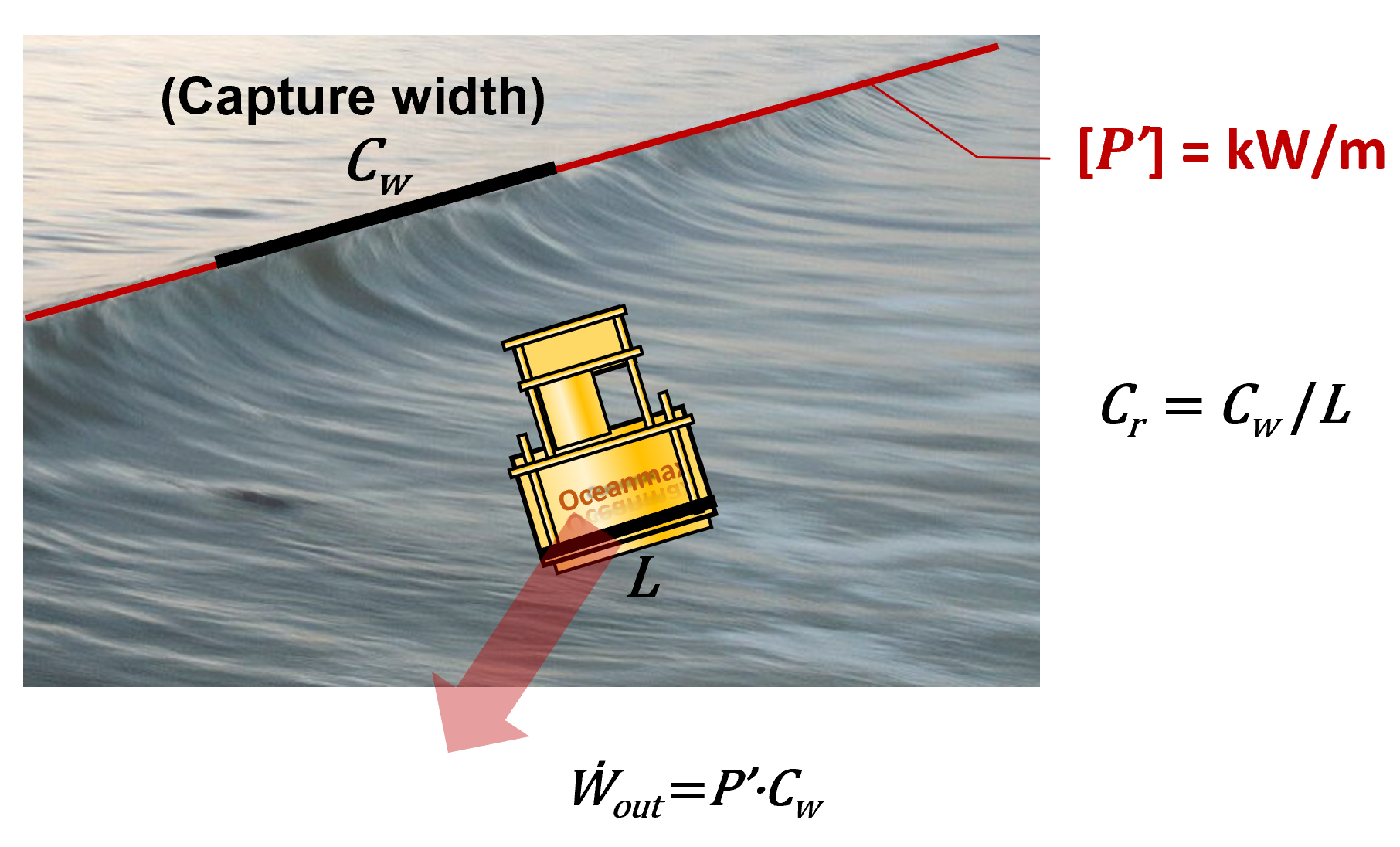
Given that there is effectively no finite amount of power that the wind contains per se, part of the problem in defining an energy conversion efficiency for a wind turbine rests in characterising the energy resource itself. Ocean energy engineering faces a similar challenge in characterising the energy content of ocean waves. To address this issue, ocean wave energy content at a specific location is typically quantified as a power per unit length of wavefront, P'. (Fig. 8.)

Furthermore, rather than an efficiency, the common measure of performance for an ocean wave energy device is capture width, C_w, the equivalent width of wavefront corresponding to the power a device generates. The larger the capture width of a device, the more power it produces, regardless of the value of the local energy resource P’. Thus, the capture width idea provides a useful measure of performance while forthrightly acknowledging the difficulty in defining a discrete amount of power input to a conversion device.

In turn, the capture width divided by the widest linear dimension of the device gives a dimensionless measure of performance, the relative capture width, C_r. Relative capture width measures the power produced by an ocean energy device relative to its size. It also allows us to compare the performance of devices of different dimensions and with different principles of operation. A minimum relative capture width of three or greater is often cited as a guideline for the potential success of a design [2]. Also pointed out in [2] is that since the relative capture width is often greater than one, it is not helpful to consider it an efficiency.

3. 2. Power Coefficient as Relative Capture Area

The wind energy analogue of power per unit length of ocean wavefront is referred to as the power density of the wind. (Fig. 9.) As opposed to power per unit length, the power density is expressed as power per unit area [5],

Likewise, we can characterize the output of a wind turbine in terms of how much of the wind power density it captures expressed as an area,

where we refer to A_cap as the turbine’s capture area. Like the capture width for ocean energy devices, the capture area of a wind turbine by itself is a useful measure of performance in that the larger its value, the more power the turbine produces regardless of the local wind energy density.

Finally, the capture area divided by the area of the actuator disc A_t defines the relative capture area, which measures the amount of wind power density captured by a turbine relative to its size. Equations 3, 4, 14, and 15 are easily rearranged to show that relative capture area is identically equal to the power coefficient:

Equation 16 gives an alternate and completely equivalent definition of the power coefficient for wind turbines. Just as the traditional definition of power coefficient of Eq. 4 does not require us to make use of any of the assumptions of linear momentum theory for its validity, neither does the alternate definition of Eq. 16. The idealised performance associated with linear momentum theory serves as a useful basis for comparison for the operation of real HAWTs regardless of the way in which power coefficient is interpreted.

4. Discussion: Advantages of the Relative Capture Area Interpretation

The interpretation of power coefficient as a relative capture area offers several advantages over the efficiency interpretation. Primarily, it avoids the ambiguity of what constitutes an input to the device by more cleanly identifying the available energy resource as the wind power density as opposed to the “power in the wind.” The relative capture area interpretation provides a great advantage in this explicit acknowledgement of the true nature of the supply of wind energy.

Quantifying the available power to a turbine as the power in the wind makes for a perplexing situation in which a resource is treated in part as a function of the device designed to harness it. This is because P_wind depends on both P” and the physical size of the turbine. Use of the correct conversion efficiency of Eq. 12 actually fairs worse in this regard, as the legitimate power input P_in=½ρA_iV_i³ also depends on the inlet area of the stream tube A_i. This area in turn depends on the size of the wind turbine and its variable operating conditions. By contrast, wind power density is a function only of geographical location at a certain point in time.

That power density represents the appropriate framing of the wind as an energy resource is reflected in the steady increase in size of turbine designs over the past forty years. In that time, turbine blade length has increased by a factor of ten, which corresponds to an increase in actuator area by a factor of 100. Non-coincidentally, the power generated by wind turbines has also increased by roughly a factor of 100 in the same time period, going from 55 kW in 1981 to 5.6 MW in 2019 [6], a clear indication of an effort to increase capture area. Furthermore, increased rotor size and hub heights are also meant to expose turbines to the higher wind speeds further up in the atmospheric boundary layer and therefore avail themselves of the larger power densities there. The increase in rated power of wind turbines is thus driven by increases in both capture area and power density.

In recognition of the resource of wind energy being a power density, both capture area and relative capture area serve as obvious measures of performance. For any turbine, we wish the capture area to be as large as possible, thereby maximizing power output for a given P”. When considering relative capture area, the actuator area A_t is indicative of the turbine’s size, and thus, its total direct cost including both capital and operational costs [8]. For two turbines with the same value of A_cap, then, we prefer the one with the larger relative capture area, as it offers us the more economical option for the same performance even if it operates at a smaller conversion efficiency.

The importance of capture area is also reflected in the U.S. industry trend of recent years towards new wind plant construction in sites of lower average wind speeds. With the smaller average power densities encountered in such sites, the push has been towards turbine designs with lower specific power, or nameplate turbine power divided by rotor swept area [7]. Energy costs are reduced via control strategies that maximize C_P at below rated speeds, leading to overall increases in turbines running near full capacity. For this strategy to work, capture area must be increased in order to account for the decreased power density at low wind speeds while simultaneously maintaining or increasing captured power. At conditions above rated wind speed, capture area is effectively decreased by pitching the blades to reduce aerodynamic loads, thereby maintaining rated power at higher power densities.

We may also argue that relative capture area is the preferred measure of performance over any energy conversion efficiency, regardless of how it is defined, in that it better aligns with the objective of the device. As an illustration of this point, we may consider the contrast between fuel economy and thermal efficiency in motor vehicles. In internal combustion engines, thermal efficiency is often highest at full throttle, indicating that the largest conversion of chemical energy into mechanical power occurs at the vehicle’s top speeds. Given that air drag scales with the square of vehicle speed, however, operating at very high speeds leads to smaller distances travelled for the same amount of fuel consumed. Hence, if our objective is to travel as long a distance as possible per unit energy consumed, we may be willing to forgo always operating at the engine’s highest thermal efficiency [9].

Lastly, since C_P is not a true conversion efficiency, we need not limit its value to between zero and one. This is an important point when we consider wind turbine designs that seemingly surpass the Betz limit, such as HAWTs that include shrouds as outlined in [10]-[12]. The shrouds, usually in the form of diffusers, increase pressure drop across the actuator disc and thus increase mass flow. This results in power coefficients that are 2-5 times larger than traditional designs and therefore values that sometimes surpass unity. In [13] it is suggested that although the cited power coefficients are legitimate, they cease to be efficiencies for shrouded turbines. A correction to the power coefficient that effectively adjusts P_wind to account for the increased mass flow is suggested, thereby reinstating the power coefficient’s alleged status as conversion efficiency, and once again recognizing the Betz limit as its maximum value.

If we abandon the idea of power coefficient as conversion efficiency to begin with, however, such adjustments become moot. A relative capture area greater than unity simply means that the effective area of wind power density captured by a HAWT is larger than its frontal area. Though a traditional, unshrouded HAWT may have an upper limit of C_P._,max = 16/27, it does not follow that other designs with different operating principles are necessarily so constrained. That being the case, power coefficient as relative capture area becomes the common measure of performance for both shrouded and unshrouded designs, and for all other wind turbines as well, including vertical axis designs and drag machines. For a wind turbine of a given size, maximizing the relative capture area will always maximize power output, whatever the energy conversion mechanism it employs and the efficiency thereof.

4. Conclusion

In this paper we have shown that the power coefficient for horizontal axis wind turbines is best thought of as its relative capture area, a parameter comparing the equivalent area of the wind power density captured by a turbine relative to the turbine’s size. The interpretation avoids the ambiguities associated with the power coefficient’s interpretation as an energy conversion efficiency, better aligns with the objectives of operating wind turbines, and also serves as a common measure of performance for all wind turbines regardless of construction and operating principle.

References

[1] A. Betz, “Das Maximum der theoretisch möglichen Ausnützung des Windes durch Windmotoren,” Zeitschrift für das gesamte Turbinenwesen, vol 26, pp. 307-309, 1920.
[2] J. Twidell and T. Weir, Renewable energy resources, 3rd ed. London, England: Routledge, 2015. View Article
[3] B. K. Hodge, Alternative Energy Systems and Applications, 2nd ed. Nashville, TN: John Wiley & Sons, 2017.
[4] M. Ragheb and R. A. Ragheb, “Wind Turbines Theory - The Betz Equation and Optimal Rotor Tip Speed Ratio,” in Fundamental and Advanced Topics in Wind Power, R. Carriveau, Ed. London, England: InTech, 2011, pp. 19–38. View Article
[5] J. F. Manwell, J. G. McGowan, and A. L. Rogers, Wind Energy Explained: Theory, Design and Applications, 2nd ed. United Kingdom: Wiley, p. 33, 2009. View Article
[6] V. Smil. “Wind Turbines: How Big?” IEEE Spectrum, vol. 56, no. 11, p. 20, 2019. View Article
[7] R. H. Wiser, M. Bolinger, B. Hoen, D. Millstein, J. Rand, G. L. Barbose, N. R. Darghouth, W. Gorman, S. Jeong, A. D. Mills, and B. Paulos. Land-Based Wind Market Report: 2021 Edition. United States, 2021. View Article
[8] G. Sieros, P. Chaviaropoulos, J. D. Sørensen, B. H. Bulder, and P. Jamieson. “Upscaling wind turbines: theoretical and practical aspects and their impact on the cost of energy.” Wind energy, vol 15, no. 1, pp. 3-17, 2012. View Article
[9] P. Roura and D. Oliu, “How energy efficient is your car?,” American Journal of Physics, vol. 80, no. 588, 2012. View Article
[10] O. Igra, “Compact shrouds for wind turbines,” Energy convers., vol. 16, no. 4, pp. 149–157, 1977. View Article
[11] O. Igra, “The shrouded aerogenerator,” Energy, vol. 2, no. 4, pp. 429–439, 1977. View Article
[12] O. Y. and T. Karasudani, “A shrouded wind turbine generating high output power with wind-lens technology,” Energies, vol. 3, pp. 634–649, 2010. View Article
[13] M. Huleihil and G. Mazor, “Wind turbine power: The Betz limit and beyond,” in Advances in Wind Power, R. Carriveau, Ed. London, England: InTech, 2012, pp. 3-29. View Article