Journal of Fluid Flow, Heat and Mass Transfer (JFFHMT)

ISSN: 2368-6111

1. Introduction

Design and development of airfoils have always been a critical operation for the aviation industry. Aerodynamic analysis for airfoils, before the 1940s, was limited to 2D analytical methods using conformal transformations about a cylinder [1]. The earliest numerical methods are Finite Difference Schemes, pioneered by Richardson [2], and other potential flow based techniques. Naturally, the solutions obtained and the allowed complexity of the geometries to be optimised depended heavily on the computing power available. In parallel, the airfoils used in practice were of growing complexity and constantly evolved. In the 1930s, the National Advisory Committee for Aeronautics conducted studies on ’families’ of foils and created the four-digit and five-digit series. Airfoil design finally moved from a manual, iterative procedure to mathematically precise analytical methods around the same time. NACA has since released multiple series of foils, each with its characteristics. This study was further developed by Jacobs, who based the development of various profiles using pressure distribution arising from the boundary layer enveloping the foil. This kind of precision is fairly ubiquitous today, indicating the importance of the developing boundary layers [3].

First studied by Prandtl, Blasius and von Karmann [4], boundary layers indicate the region through which viscous effects are to be modelled. They were first solved analytically, and then numerically by the 1950s. The methods employed today rarely use the quintessential difference schemes, and eschew them in favour of more robust methods that can work with complex geometries faster. An important class of methods are the Panel methods, first outlined by Hess and Smith, 1967 [5]. These methods incorporate curved geometries using panels over the surface more easily than difference schemes and are often faster. These methods have been extensively studied and developed over the years, growing in complexity, often using multi-order methods. As a tangent, this work considers a novel extension to the prototypical flat plate solution to solve for the steady-state boundary layer of a symmetric NACA airfoil. The curved geometry of the airfoil is approximated as a series of inclined flat plates. Then, the boundary layer of each such plate is solved sequentially, where the velocity profile at the trailing edge of one plate is repurposed into the initial velocities for the next plate. The resulting velocity profiles give us the developed boundary layer.

The rest of the paper is organised as follows. The following sections detail the flat plate boundary layer and then follow into the inclined flat plate problem. The latter is then extended to curved geometries, which we test on symmetric four-digit airfoils. The approximate solutions for the velocity fields are then used to compute the coefficient of lift, which is used to verify that the method does indeed model the boundary layer over the foil.

2. Theory

The problem we have set out to solve is as follows: Given an understanding of the simple steady-state flat plate boundary layer solution originally solved by Prandtl et al., is it possible to extend the solution to curved geometries in a way that does not rely on complicated machinery i.e. on formulations beyond the flat plate solution? We pursue this solution over symmetric NACA airfoil geometries and test its range of validity. With the benefit of hindsight, we reply in the affirmative - there is such a method. However, there are some caveats. While it is possible to define and test such a method, some limitations beset it. This means that beyond a certain limit or curvature in the geometry of the foil, the solution becomes quite inaccurate and we must responsibly defer to more robust formulations.

This section develops the flat plate boundary layer solution to solve the inclined flat plate problem. This solution is then used to construct the new method, which is used to solve the boundary layer flow over curved geometries.

2.1. Background

This section introduces the notation and the required background for them.

The velocity field u(x,y) is a vector field, with x-component u(x,y) and vertical component v(x,y). Note that the vector field is always indicated with a boldface character, and that both components are functions of x and y. The aim is to solve for this field in the forthcoming sections.

In that regard, we use a finite difference scheme developed in [6], and the notation is as follows. In a Cartesian coordinate system, we use the x and y axes as usual, and the velocity at each node is denoted by capital letters. Specifically, the finite difference method calls needs a discretised domain, which we do by demarcating points along the x-axis spaced Δx apart, and Δy apart on the y-axis. The resulting grid that we form will be the basis for our finite difference scheme, and we index each node by (i,j). That is, node (i,j) corresponds to the coordinate point (iΔx ,jΔy), and it is easily seen that this can cover the domain.

The velocity field is then solved for at each node, instead of the entire, continuous domain. This is the crux of the finite element method, and we use the following notation. U_(i,j) denotes the horizontal component of velocity, u(x,y), at the (i,j) node, i.e. U_(i,j)= u(iΔx ,jΔy). Similarly, V_(i,j) denotes the vertical component of velocity, v(x,y), at the (i,j) node i.e. V_(i,j)= v(iΔx ,jΔy).

The physical constants used in the governing equations are introduced with the corresponding equations for brevity.

2.2. Boundary layer equations

The governing equations for this flow are derived from the Navier-Stokes equations, which are as follows.

where u is the x-component of the velocity field u, and v is the y-component. We will always indicate the vector velocity field as a boldfaced u. Further note that these are with respect to the global coordinate axes. When solving over each region, these will be resolved along appropriately inclined axes, and the meaning will be clear from context. Lastly, ν is the kinematic viscosity of the fluid; in this case, air. We can now simplify Eq. 1 as follows:

Subject to the following boundary conditions

We also specify mass conservation throughout as follows.

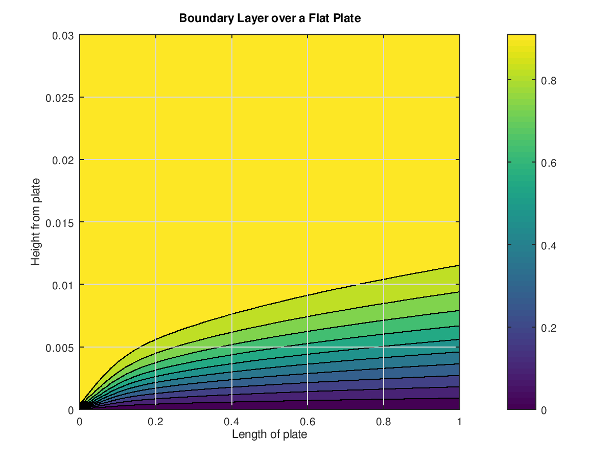
2.3. Boundary Layer over a Flat Plate

Consider a horizontal stream with velocity incident on a flat plate of negligible thickness as shown. Naturally, we are subject to the no-slip condition at the bottom of the plate, and we assume that we reach the free-stream velocity beyond the layer. These are essentially the conditions outlined in Eq. 3.

Now, we can say that the problem is well-posed. We can now begin discretizing Eq. 2. With help from [6], we use the following derivative approximations:

Recall, U_i,j denotes the steady flow velocity component at the (i,j)^th node. Following the literature in Finite Difference Methods, each node represents a point in the domain where the velocity field is resolved. Naturally, U_i+1,j refers to the node i.e. the succeeding node along the (local) x-axis, and U_i,j+1 refers to the node i.e. the succeeding node along the (local) y-axis. Note that because we deal with curved geometries, ∆x and ∆y, the node spacings along the x and y axes vary according to the curved geometry. In accordance with the literature in Finite Difference Methods, each node represents a point in the domain where the velocity field is resolved. When Eq. 5 is substituted in Eq. 2, we get

We can now rearrange this to form an equation in U_(i,j) , U_(i+1,j) and U_(i,j+1) as follows.

However, at the boundaries, we must modify our equation, which is then of the form

near the plate, and

near the edge of the domain. Now, we see that this method is implicit and thus can be resolved into a tridiagonal system to fully resolve the velocities at the j^th layer. Because this is an implicit method, it is unconditionally stable; this allows us to have arbitrary levels of discretisation in the numerical analysis.

We depict one such solution for the flat plate in Figure 1, for laminar flow using the conditions as applicable from Sec.2.3. Please note that here, we follow the surface of the plate, even if it coincides with the Cartesian x-axis. We will define our x-axes in the next sections along the curve as well.

2.4. Boundary layer over a symmetric airfoil

Any airfoil is characterised by curved geometry, which is not easily amenable to an FD method. Past methods have tried to use meshed irregular grids i.e. grids with step size that varies with geometry or even tried to remove the mesh entirely [4]. The latter is done via the random generation of nodes and using neighbouring nodes to compute the velocity. In any case, the fact remains that this difficulty in moving to complex geometries is one of the reasons for introducing more robust methods.

A key observation is that these methods depart significantly from the otherwise simple analysis outlined above. As engineers are wont to do, our method to compute the velocity field builds on the flat plate solution. We use linear splines to approximate the curved airfoil boundary as a series of flat plates, and then solve the flat plate problem over each region. The only added complexity is with the change in slope of each section, i.e. we now have to solve an inclined flat plate boundary flow problem.

Solving an inclined flat plate presents only one difficulty over the normal problem. The incoming velocity field, though horizontal, will have to be resolved along the plate. Let us suppose that the velocity fields are essentially thus: initially. Furthermore, let the slope of the plate be θ. Then, denoting [U’,V’] as the components as resolved on the plate, we can easily see that

Note that this only resolves the velocities at the first plate i.e. at the leading edge. There are more spline interpolations along the curve. Fortunately, Eq. 10 generalises easily to

where U_i denotes the incoming velocity profile at the i^th plate and so on, and θ is the difference in the slopes between the i^th and (i-1)^th plates. With these modifications, we can repeatedly use the flat plate solution as outlined in Section 2.2.

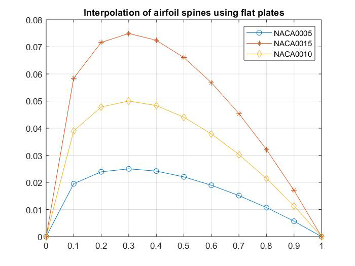
Figure 2 shows linear spline interpolations of airfoils with multiple thicknesses and zero camber, of which the 5% thickness profile was used to test this method. To reiterate, each segment of the spline will be treated as an inclined flat plate and solved thus. The velocity profiles at the ends of each plate/segment are stored as the velocities of the fluid along the foil. It is easily seen then, that a larger number of splines would result in a better approximation of the velocity profile.

We study the case when , and , i.e. a horizontal flow over a symmetric NACA 0005 foil. The fluid is assumed to be air, which gives us approximately. Further note that the foil is assumed to be smooth i.e. we neglect the wall-shear component in the following calculations.

2.5. Calculating the Lift Coefficient

Calculating the coefficient of lift, C_l gives us an important verification of the method developed here. Briefly, it is the ratio of the lift force generated by the foil to , where 𝜌 is the density of the fluid (here, air), V is the velocity of the wing and A is the frontal area of the wing. The latter can be thought of as the area exposed to the incoming velocity.

The coefficient of lift has to be calculated using the velocity profiles over each individual plate. Note that the coefficient of lift is calculated as follows. To find the lift force L, note that for an individual segment of length Δl

where V_u denotes the boundary layer velocity when developed over the upper segment of the foil, V_lis the same velocity developed on the lower segment, and b is the depth of the plate. ΔP indicates the differential pressure across the length of the foil. For simplicity, we ignore any fringe effects. Now, we can sum over all the plates to get the total lift force for the foil

Therefore, we can use the definition of C_l as follows.

Finally, assuming the mean velocities V_l and V_u, we get

where , and for some . Using the approximation detailed above, we obtain the computed values of C_l as shown in Table 1. Their close agreement allows us to see that the method developed does indeed model the foil accurately. The theoretical values are derived from Eq. 16 from Thin Airfoil theory.

where α is the angle of attack, and C_l is the lift coefficient.

The authors, however, recommend that Eq. 15 only be used when a rough estimate is required. The equality in Eq. 14 yields calculations of the lift coefficient that conform to the theoretical values; this, we suspect, may be because the inequality is not tight.

3. Results

Using this solution, accuracy is compared with traditional Thin Airfoil Theory and the characteristics of the obtained velocity field.

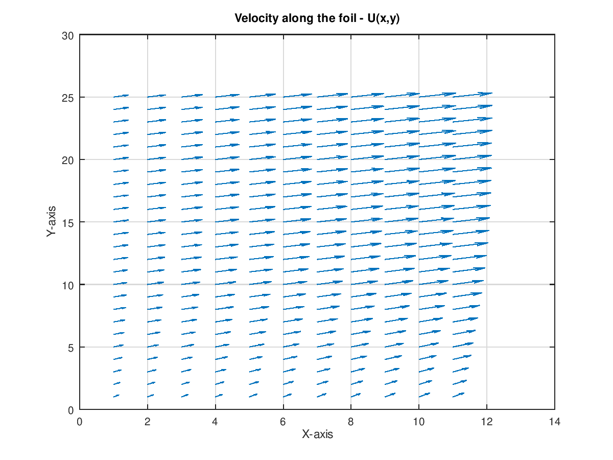
The obtained velocity field for the conditions described at the end of Section 2.4. is shown in Figure 3. It is important to note the graph precisely, however. The x-axis follows the curve of the foil, and this means that two points shown at the same height on the graph are in fact at the same height from their corresponding points on the foil, but not in the sense of an orthogonal Cartesian coordinate system measured from the nose of the foil. Having presented this way, we can easily see the developing boundary layer as if we were following a flat plate. Visually, we can see that the boundary layer does not separate, which is to be expected for the laminar flow we have considered. This serves as the first verification of our framework.

The other confirmation comes from the computation of the coefficient of lift (C_L) for different values of angles of attack (α) and comparing it with the predicted values from Thin Airfoil Theory. To obtain the coefficient of lift from the velocity field, we proceed in a two-part computation.

Consider the foil as made up of two halves, each made up of the surfaces of the top and bottom of the foil respectively. Since we consider the symmetric NACA 0005 airfoil, we do not need to account for different geometry in each step. Now, the crucial part is to account for the angle of attack (α), which we do as follows. Prior to resolving the flow along any of the individual plates, we angle the flow according to ɑ. That is, , where R(-α) is the rotation matrix as described in Eq. 11 for an angle of -α . Note, however, that for a positive angle of attack, we incline the flow in the opposite sense. This is, in effect, giving us the scenario when the foil is inclined by +α. . Then, we calculate the velocity field as shown in Sections 2.3 and 2.4, and find the boundary layer velocity for the upper half, V_u.

We repeat this procedure for the lower half of the foil, noting that the geometry does not change for symmetric foils. We incline the initial flow to +α, as opposed to (-α) in the previous part. This allows us to simulate the flow as if the foil was inclined away from it. We proceed similarly as before and calculate the boundary layer velocity for the lower half, V_L.

An approximate upper-bound calculation is used to find the lift coefficient, C_l, from V_u and V_L, as detailed in Section 2.5. The accuracy of the method can be now easily determined by a computation of the total lift force that the foil creates, as listed in Table 1. As Table 1 shows, the close agreement with the calculated and predicted values serves as the final verification of our framework.

Table 1. Approximate upper bound of lift coefficient vs actual lift coefficient in a NACA 0005 Airfoil with various angles of attack.

Angle of attack (α)	Approx. Coefficient of Lift (C'l)	Theoretical Coefficient of Lift (Cl)
2°	0.24	0.219
4°	0.43	0.438
6°	0.67	0.657
8°	0.76	0.87
10°	0.80	0.6

4. Conclusion

The inclined flat plate boundary layer solution is sequentially applied, piecewise, to approximate the flow-field over a curved airfoil. The lift coefficient is obtained from the flow-field so calculated, and values obtained closely match well established results. The deviation, however, increases at higher angles of attack, owing to inherent simplifications in the method. Furthering the work done so far, the authors propose to quantify approximation errors, which can then be used to extend the method to more complex geometries such as cambered airfoils, and at larger angles of attack.

References

[1] L. M. Milne-Thomson, Theoretical aerodynamics. Courier Corporation, 1973.
[2] W. Covey, “Weather prediction by numerical process: By Lewis F. Richardson, Dover Publications, Inc. paperback. 1965.,” Soil Science Society of America Journal, vol. 30, no. 1, pp. vi–vi, 1966. View Article
[3] E. N. Jacobs, K. E. Ward, and R. M. Pinkerton, The Characteristics of 78 Related Airfoil Section from Tests in the Variable-Density Wind Tunnel. No. 460, US Government Printing Office, 1933.
[4] T. Liszka and J. Orkisz, “The finite difference method at arbitrary irregular grids and its application in applied mechanics,” Computers and Structures, vol. 11, no. 1-2, pp. 83–95, 1980. View Article
[5] J. L. Hess and A. Smith, “Calculation of potential flow about arbitrary bodies,” Progress in Aerospace Sciences, vol. 8, pp. 1–138, 1967. View Article
[6] F. Blottner, “Finite difference methods of solution of the boundary-layer equations,” AIAA journal, vol. 8, no. 2, pp. 193–205, 1970. View Article