Journal of Fluid Flow, Heat and Mass Transfer (JFFHMT)
ISSN: 2368-6111

Volume 8 - Year 2021 - Pages 80-92
DOI: 10.11159/jffhmt.2021.010
An Artificial Compressibility Based Approach to Simulate Inert and Reacting Flows
Mariovane Donini1, Fernando Fachini1, Cesar Cristaldo2,
Pascal Bruel3
1Grupo de Mecaˆnica de Fluidos Reativos
Instituto Nacional de Pesquisas Espaciais, 12630-000 Cachoeira Paulista-SP, Brazil
mariovane.donini@inpe.br; fernando.fachini@inpe.br
2Laboratório de Fluidodinâmica Computacional e Turbulência Atmosférica
Universidade Federal do Pampa, 97546-550 Alegrete-RS, Brazil
cesarcristaldo@unipampa.edu.br
3CNRS - University Pau & Pays Adour, LMAP
Inria Cagire Team, Av. de l’Universite´, 64013 Pau, France
pascal.bruel@univ-pau.fr
Abstract - An efficient methodology to simulate non-reactive and reactive flows is presented. Combining a finite-volume approach on fully staggered meshes along with the artificial compressibility method, the resulting code proves to be versatile enough to cope with flow configurations ranging from unsteady cylinder wakes, heated cylinder or steady and unsteady diffusion flames with excellent accuracy, in the limits of the underlying physical modelling.
Keywords: Mach zero framework, finite volume, fully staggered mesh, steady flows, unsteady flows, diffusion flames.
© Copyright 2021 Authors - This is an Open Access article published under the Creative Commons Attribution License terms Creative Commons Attribution License terms. Unrestricted use, distribution, and reproduction in any medium are permitted, provided the original work is properly cited.
Date Received: 2020-11-30
Date Accepted: 2021-12-04
Date Published: 2021-02-19
1. Introduction
The artificial compressibility (AC) method is quite a well-established numerical approach for solving the constant-density incompressible Navier-Stokes equations. Originally introduced by Chorin [1] for steady flows simulations, this method consists in that case in modifying the continuity equation by adding a non-stationary pressure term, namely:
where ![]() is a an artificial e.g. non-physical time and
is a an artificial e.g. non-physical time and ![]() is the artificial compressibility factor which scales as a velocity square. In the following and unless stated otherwise, any quantity
is the artificial compressibility factor which scales as a velocity square. In the following and unless stated otherwise, any quantity ![]() is dimensional whereas its dimensionless counterpart is written as
is dimensional whereas its dimensionless counterpart is written as ![]()
The results are physically meaningful only when a steady-state solution in τ is reached so that the original continuity equation is recovered [2]. The ongoing popularity and relative success of the artificial compressibility method to deal with constant density flow simulations are mainly due to its simplicity and clear physical interpretation. To obtain a time-accurate solution, a dual time-step technique can be employed [3, 4, 5, 6]. Accordingly, in addition to the aforementioned modification of the continuity equation, the physical time derivative of the velocity field is introduced in the momentum equation, namely (dimensionless form):

where t is the physical time, Re the Reynolds number, ∂t and ∂τ are the physical and artificial-time derivatives, respectively. These equations are iteratively solved such that the velocity field approaches its new value in physical time as its divergence is driven towards zero. Thus, for each physical time step, the flow field has to go through one complete sub-iteration cycle in artificial-time.
The existence of the artificial-waves propagation phenomenon associated with the convergence towards the physically meaningful solution of the above set of equations can be evidenced by writing the momentum equation under a characteristics-like form (neglecting the viscous term and the physical time derivative and considering a one-dimensional configuration), namely:

The artificial sound speed c, and the corresponding artificial Mach number M, are related to β by:
Thus, artificial waves of finite speed are introduced to distribute the static pressure throughout the whole computational domain. The rate of convergence of the solution during the pseudo-time integration loop heavily depends on the value of β, and this can be thought of as a weak point of the method. Indeed, in order to converge to the steady-state solution during the course of each sub-iterations cycle in artificial-time, the waves associated to the hyperbolic nature of the artificial compressibility based system of equations have to undergo at least a one round-trip propagation to ensure the proper built-up of the pressure field (more precisely, of its gradient field) over the whole computational domain. Based on this representation, Chang and Kwak [6] estimated the number N of artificial time-steps Δτ required to reach convergence in artificial time. By considering a characteristic length L of the computational domain over which the artificial waves must travel once forth and back, they obtained a lower bound for N expressed as:
Compared to the numerous AC based simulations of constant density flows that can be found in the literature (quite a significant number of them have been recently recalled by Hodges [8]), much less examples of AC based simulations of non-constant density flows have been reported or are discussed in CFD textbooks, to the noticeable exception of Oran and Boris [9]. In such cases featuring a non-constant density field (in space and/or in time), one can distinguish between configurations still featuring a divergence free velocity field (Bassi et al. [10], Shapiro and Drikakis [11]) from those which did not. For the latter, they are mostly related to the simulation of Mach zero reacting flows such as steady turbulent premixed flames (Bruel et al. [2]), unsteady turbulent premixed flames (Corvellec et al. [5], Dourado et al. [7]), laminar confined and unconfined diffusion flames (Fathi et al. [12], Bianchin et al. [13], Donini et al. [14]).
Starting from the observation that the artificial compressibility is quite underused to simulate in particular reacting flows, the objective of the present work is to draw the attention of the CFD community on this valuable approach by showing how the combination of rather standard discretization tools in a finite volume framework allows to obtain an efficient and versatile simulation tool. In addition to the Introduction and Conclusion sections, the paper is organized in three main sections: Section 2 describes the different continuous systems of equations to be solved; Section 3 gives the main ingredients of the methods of solution whilst in Section 4, the results obtained for five different flow configurations are presented.
2. The Continuous Systems of Equations
Both inert and reacting gaseous flows are to be considered in the present study and the possible influence of the buoyancy force is accounted for. Thus, for each of the two classes of configurations, the modified (e.g. including the AC related terms) continuous system of equations dealt with is presented hereafter. 2D flow geometries are considered in this study, either in Cartesian or axisymmetric coordinates.
2. 1. Inert Flows
A Newtonian fluid is considered for which the modified conservation equations of mass, momentum and energy are given by:


Where ![]() designates the dimensionless velocity vector,
designates the dimensionless velocity vector, ![]() is the viscous stress
tensor and the power-law expressions
is the viscous stress
tensor and the power-law expressions ![]() (with
(with ![]() ) are employed to account for the temperature
dependence of he shear viscosity
) are employed to account for the temperature
dependence of he shear viscosity ![]() and thermal diffusivity
and thermal diffusivity ![]() . Vector
. Vector ![]() stands for the base vector aligned with
the gravity acceleration vector
stands for the base vector aligned with
the gravity acceleration vector ![]() . The dimensionless variables and differential operator are defined as:
. The dimensionless variables and differential operator are defined as: ![]() ,
, ![]() ,
, ![]() ,
, ![]() ,
, ![]() ,
, ![]() ,
, ![]() and
and ![]() ,
, ![]() . The reference quantities used to define the
Reynolds number
. The reference quantities used to define the
Reynolds number ![]() , the Froude number
, the Froude number ![]() and the Péclet number
and the Péclet number ![]() (with
(with ![]() ,
, ![]() , where
, where ![]() is the reference dynamic viscosity,
is the reference dynamic viscosity, ![]() the reference thermal diffusivity
the reference thermal diffusivity ![]() the thermal conductivity and
the thermal conductivity and ![]() the reference specific heat at constant pressure) will be
indicated later on, on a case by case basis. The above system is supplemented
by the Mach zero equation of state, namely
the reference specific heat at constant pressure) will be
indicated later on, on a case by case basis. The above system is supplemented
by the Mach zero equation of state, namely ![]() . When the flow configuration dealt with is
isothermal, the energy equation simply reduces to T=cste
. When the flow configuration dealt with is
isothermal, the energy equation simply reduces to T=cste
2. 2. Reacting Flows
Two different diffusion flames in ambient atmosphere are simulated to illustrate the capability of the AC method to deal with reacting flows with a strongly varying density. They are both described through a simple thermochemical model. It assumes an infinitely fast one-step chemical reaction i.e. F+s O2→(1+s) P (At stoichiometry, s mass of oxygen is consumed for each unit mass of fuel F resulting in 1+s mass of products P). Thus, the temperature T and the mass fraction fields Yi (i=O2, F) are determined by two conserved scalars [19, 20, 21]: the mixture fraction Z≡S YF-YO2+1 and the excess enthalpy H≡(S+1) T/Q+YF+YO2 in which ![]() and
and ![]() where
where ![]() and
and ![]() are the reference mass fraction of fuel and mass fraction of oxidant, respectively, which supplement the reference quantities already introduced in the previous subsection for inert flows. Q is the heat of combustion. Both fuel and oxidant Lewis numbers are taken equal to unity. Thus, the generic system of governing equations that describes the evolution of the reacting flows at hand is given by:
are the reference mass fraction of fuel and mass fraction of oxidant, respectively, which supplement the reference quantities already introduced in the previous subsection for inert flows. Q is the heat of combustion. Both fuel and oxidant Lewis numbers are taken equal to unity. Thus, the generic system of governing equations that describes the evolution of the reacting flows at hand is given by:


The above system is supplemented by the Mach zero equation of state, namely ρ=1/T.
3. Method of Solution
The numerical solution of the Mach zero system of equations relies on a dual-step time-accurate artificial compressibility method. An explicit second-order Runge-Kutta Ralston’s method was adopted for the artificial-time integration and the second-order Euler method was selected for the physical-time integration due to its simplicity of implementation in a dual-time step approach.
By replacing the derivative terms with their numerical approximations, the resulting set of equations can be written in compact form as:
where q=[ρ,u,v,T]T and q(ac)=[p/β,u,v,T]T are the vector of primitive variables for non reacting flows, and q=[ρ,u,v,Z,H]^T and q(ac)=[p/β,u,v,Z,H]T are those for reacting flows cases. RHS(q)i,j is the right-hand side of the discretized equation. Then, introducing the residual value for the artificial time step as:
permits to rewrite Equation 13 at times’ step (𝑛+1,𝜈+1) as:
The integration steps in artificial-time are finally given by:


where (α1,α2,α3 )=(1,3/4,1/3), (ϕ1,ϕ2,ϕ3 )=(1,1/4,1/3) and ΔΩ is the cell volume.
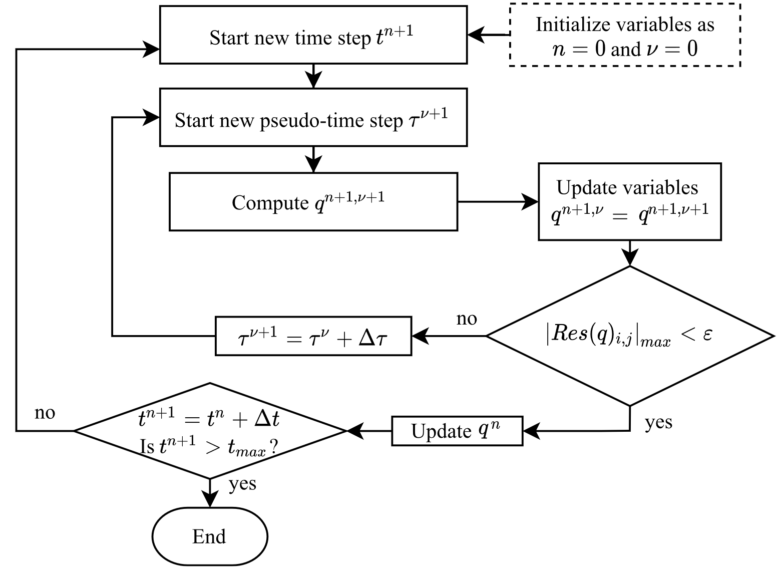
To advance the solution by one physical time-step, the equations are iteratively solved in a segregated way such that qn+1,ν+1 approaches the new value qn+1 as the artificial time derivative approaches zero. For satisfying this constraint, the residual value Res(q)i,j of Equation 15 is set to reach values below ε= 10-5. The flow chart of the algorithm to solve the system is presented in Figure 1.
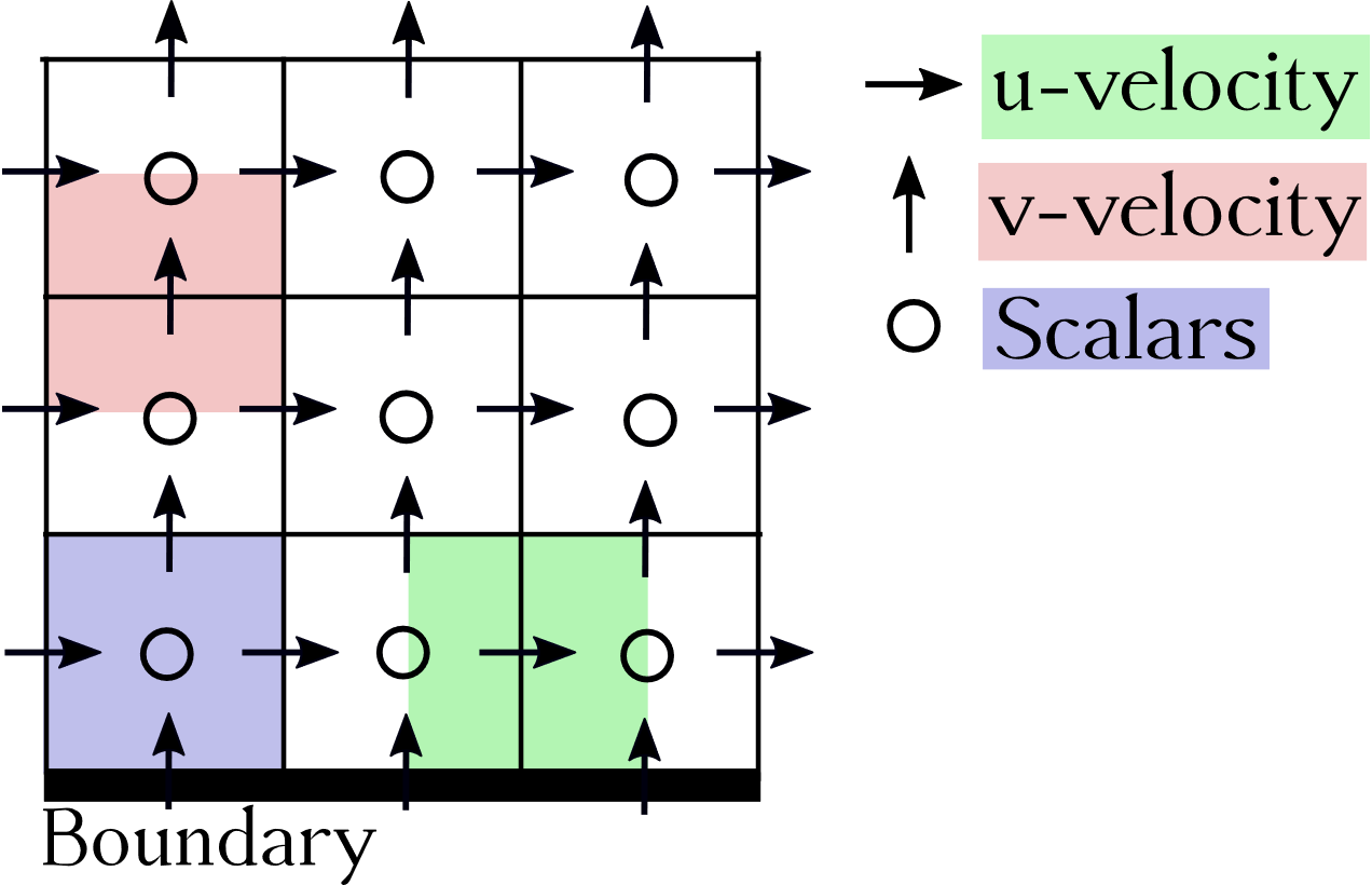
A finite volume framework is adopted. The governing equations are discretized on a staggered grid by a cell-vertex finite-volume formulation using the quadratic upstream interpolation for convective kinetics (QUICK) scheme to guarantee stability, sensitivity to the flow direction and third-order truncation error. There is no need to prescribe boundary conditions for the pressure, thanks to the recourse of the fully staggered grid, as shown in Figure 2. The non-uniform structured grid is refined (hyperbolic tangent distribution), on a case by case basis, in zones where high gradients are expected.
4. Numerical Experiments
A total of five flow configurations were simulated broken down into i) three inert flow configurations (two isothermal and one featuring a strongly space varying density) and ii) two reacting flow configurations (one steady laminar diffusion flame and one flickering laminar diffusion flame).
4. 1. Inert Flows
Three different inert flow configurations are considered. The first one (the oscillating plate) is a verification test aimed at assessing the effective accuracy of the method of solution. The two others are validation tests that demonstrate the capacity of the method to cope with flow featuring unsteady vortices (unsteady cylinder wake) or strong density variation (a heated cylinder placed in a square enclosure).
4. 1. 1. The Oscillating Plate (Stokes’ Second Problem)
The flow motion over an infinite flat plate that oscillates parallel to itself is investigated. The coordinate system is 2D Cartesian, with x ̂ being the coordinate along the plate and y ̂ the coordinate normal to it. The plate oscillates in the y ̂=0 plane with a velocity given by:

![]() designates the plate oscillation frequency and
designates the plate oscillation frequency and ![]() the time. The fluid is air and the reference kinematic viscosity is taken at ambient temperature e.g.
the time. The fluid is air and the reference kinematic viscosity is taken at ambient temperature e.g. ![]() . The maximum plate velocity is taken as the reference velocity e.g.
. The maximum plate velocity is taken as the reference velocity e.g. ![]() and the reference length is chosen equal to eight times the depth of penetration of the viscous wave e.g.
and the reference length is chosen equal to eight times the depth of penetration of the viscous wave e.g.![]() . Thus, the Reynolds number is such that Re=64. The fluid velocity is given by (Schlichting [18]):
. Thus, the Reynolds number is such that Re=64. The fluid velocity is given by (Schlichting [18]):

where where ![]() . The global error at time level n will be denoted by
. The global error at time level n will be denoted by ![]() , where
, where ![]() is the computed value at each point of the grid and
is the computed value at each point of the grid and ![]() represents the exact value.
represents the exact value.
To quantify the error, the commonly used p-norm is chosen in order to estimate the error at a given physical time level n, namely:
Let’s assume the method has an order of accuracy s, then the error is expected to behave like ‖En ‖p=C(Δt,Δy)s+ high-order-terms, as the time step or grid spacing are decreased and (Δt,Δy)→0.
Figure 3 shows the results of the time step and mesh refinement influence study for the Stokes' second problem using the p-norm with p=1. The exact and computed solutions are compared on a sequence of time steps and grid spacing, and the norm of the error is plotted as a function of Δt and Δy. These are shown on a log-log scale, e.g. log ![]() so that a linear behaviour is expected in this plot, with the slope providing the effective order of accuracy s. When decreasing Δt, the mesh refinement is adapted in order to keep constant the Courant–Friedrichs–Lewy number at the value CFLt=0.5
so that a linear behaviour is expected in this plot, with the slope providing the effective order of accuracy s. When decreasing Δt, the mesh refinement is adapted in order to keep constant the Courant–Friedrichs–Lewy number at the value CFLt=0.5
4. 1. 2. The Unsteady Wake of a Flow past a Circular Cylinder
The incompressible unsteady laminar flow around a cylinder with a circular cross section of diameter ![]() placed eccentrically in a channel of height
placed eccentrically in a channel of height ![]() is considered (see Figure 4). The coordinate system is 2D Cartesian, with
is considered (see Figure 4). The coordinate system is 2D Cartesian, with ![]() being the streamwise coordinate and
being the streamwise coordinate and ![]() the coordinate normal to the channel walls. This configuration corresponds to one of those used by Schafer and Turek [16] for a benchmark of different solution approaches for solving the incompressible Navier-Stokes equations. The distances between the cylinder centre and the bottom and top walls are
the coordinate normal to the channel walls. This configuration corresponds to one of those used by Schafer and Turek [16] for a benchmark of different solution approaches for solving the incompressible Navier-Stokes equations. The distances between the cylinder centre and the bottom and top walls are ![]() and
and ![]() , respectively. The Reynolds number is defined by
, respectively. The Reynolds number is defined by ![]() , where
, where ![]() is the kinematic viscosity and
is the kinematic viscosity and ![]() denotes the bulk velocity. The case selected here corresponds to Re=100. As illustrated in Figure 4, Equations 6 and 7 are integrated with the following boundary conditions: on the top
denotes the bulk velocity. The case selected here corresponds to Re=100. As illustrated in Figure 4, Equations 6 and 7 are integrated with the following boundary conditions: on the top ![]() and bottom
and bottom ![]() walls and at the cylinder surface (r2=x2+y2) the no-slip condition is imposed for velocities. At the inlet section located at
walls and at the cylinder surface (r2=x2+y2) the no-slip condition is imposed for velocities. At the inlet section located at ![]() , a parabolic profile is prescribed for the velocity streamwise component (with a maximum value
, a parabolic profile is prescribed for the velocity streamwise component (with a maximum value ![]() ) and the normal component is set to 0.
) and the normal component is set to 0.
Among all the characteristics of this type of problem (lift, drag, and pressure coefficients), the correct prediction of the periodic vortex-shedding, illustrated by the isocontour of velocity in Figure 5c was the target chosen to validate the present solution approach. In particular, the Strouhal number is computed to measure the ability of the method to produce quantitatively accurate unsteady results. Figure 5a presents the time evolution of the non-dimensional normal component of the velocity at (x,y)=(-0.5,0.5) observed when the periodic regime of shedding is established. For Re=100, the experimentally obtained Strouhal number is St=0.287±0.003 [16]. The power spectrum of the fluctuations of the streamwise component of the computed velocity is shown in Figure 5b. The numerically obtained Strouhal number value is St = 0.289 which agrees well (relative error of 1.35%) with its experimentally obtained counterpart. For the present case, Figure 6 shows, for a given physical time-step, an evolution of the maxima of the residuals Res(v)i,j (Equation 15) during the artificial-time iteration cycle.
It can be seen that calculations for β=40 become unstable and within 40 steps starts to diverge, whereas other cases converge to a stable solution. For low values of β, it takes only 10 iterations for the solution to reach almost constant residual values but then, further iterations do not improve the solution and so the accuracy constraint cannot be met. The effect of the artificial compressibility factor β on the number of artificial-time steps necessary to achieve convergence to the physical time step following that corresponding to the snapshot of Figure 5c is illustrated in Figure 7. L is defined as the channel length and Δτ=0.14. The optimum value of βopt≈34 is higher than the expected value of βopt≈8 reported in the literature [2, 11]. By using Equation 5, the dashed line in Figure 7 represents the number of minimum time-steps to achieve convergence of the artificial-time integration for each value of β. Considering the convergence criteria of Res(v)max<ε, it is possible to see a good agreement between the computation iterations and the iterations described by Equation 5 until βopt.
For β>βopt, the convergence rate begins to degrade gradually until β≈38, above which convergence is lost.
4. 1. 3. A Square Enclosure with a Heated Circular Cylinder
The configuration is 2D Cartesian. It consists of a cooled square enclosure kept at a constant temperature ![]() , with sides of length
, with sides of length ![]() , within which a heated circular cylinder at constant temperature
, within which a heated circular cylinder at constant temperature ![]() with a radius
with a radius ![]() , is located in the center of the enclosure. This configuration was studied by Kim et al. [22] to examine the natural convection phenomena by changing the location of the circular cylinder. The case selected here corresponds to
, is located in the center of the enclosure. This configuration was studied by Kim et al. [22] to examine the natural convection phenomena by changing the location of the circular cylinder. The case selected here corresponds to ![]() ,
, ![]() and
and ![]() so that the Rayleigh number defined as
so that the Rayleigh number defined as ![]() with
with ![]()
![]() is such that Ra=10^3, leading to reference values
is such that Ra=10^3, leading to reference values ![]() and
and ![]() . The hot cylinder and cold wall temperatures are such that
. The hot cylinder and cold wall temperatures are such that ![]() < and
< and ![]() , respectively.
, respectively.
Once the velocity and temperature fields are obtained, the local Nusselt number Nu and the surface-averaged Nusselt number ![]() are defined as:
are defined as:
Where ![]() , n is the normal direction with respect to the walls and K is the wall surface area over which the integration is performed.
, n is the normal direction with respect to the walls and K is the wall surface area over which the integration is performed.
The Nusselt numbers results presented by Kim et al. [22] were used to evaluate the efficacy of the present solution approach. Figure 8 present the predicted flow topology streamlines. This topology highlights the buoyant induced flow, caused by the upward motion of the hot fluid that moves along the surface of the heated cylinder. The hot fluid then encounters the cold top wall becoming gradually colder and denser while it moves horizontally outward of the vertical center line. At this stage, the fluid is cold enough to descend along the cold side walls closing the recirculation zone. Figure 9 displays the distribution of the local Nusselt number along half of the wall of the enclosure. Because the problem presented symmetry about the vertical center line at x=0, only the right half of the enclosure is considered (see Figure 9) for calculating ![]() . The present simulation yields a value
. The present simulation yields a value ![]() which is within 3.59 %. of that reported by Kim et al. [22] e.g.
which is within 3.59 %. of that reported by Kim et al. [22] e.g. ![]() .
.
4.2. Reacting Flows
4.2.1 Tsuji Burner Flame
This configuration is concerned with the flame stabilization over a porous cylindrical burner with radius ![]() inside a channel. The geometry is 2D Cartesian. As shown in Figure 10, the gaseous fuel is injected from the forward half part of the burner with velocity
inside a channel. The geometry is 2D Cartesian. As shown in Figure 10, the gaseous fuel is injected from the forward half part of the burner with velocity ![]() into the incoming airflow of velocity
into the incoming airflow of velocity ![]() .
.
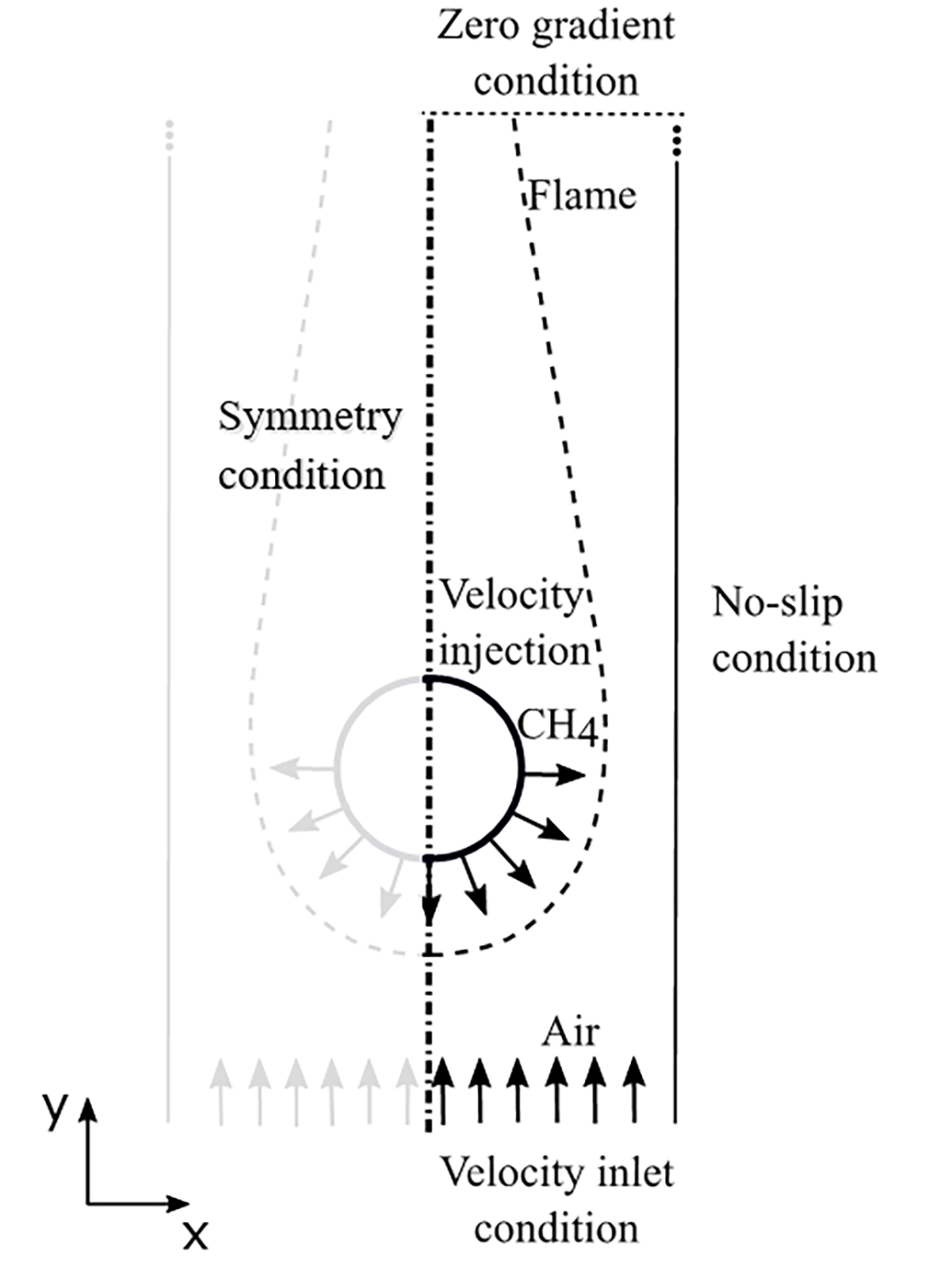
This configuration reproduces the experimental set-up of the Tsuji Burner, where the rear side of the burner surface was coated to avoid the ejection of fuel into the wake region [17]. In such a configuration characterized by a low incoming flow velocity, an envelope steady flame is found. The flame is described by the set of Equations 9-12 where the other reference quantities are chosen as ![]() ,
, ![]() ,
, ![]() ,
, ![]() and
and ![]() where the index b and ∞ denote quantities taken at the burner exit and in the ambient atmosphere, respectively.
where the index b and ∞ denote quantities taken at the burner exit and in the ambient atmosphere, respectively.
Equations 9 to 12 are integrated with the
following boundary conditions: On the symmetry axis ![]() ,
, ![]() ; at the burner boundary surface
; at the burner boundary surface ![]() ,
, ![]() ,
, ![]() ,
, ![]() (Robin’s like boundary type for
(Robin’s like boundary type for![]() and
and ![]() ) where
) where ![]() ,
, ![]() and the subscript
and the subscript ![]() stands for the
normal to the burner surface. The terms
stands for the
normal to the burner surface. The terms ![]() and
and ![]() are the
are the ![]() and
and ![]() fluxes which are imposed at the burner injection
surface
fluxes which are imposed at the burner injection
surface
![]() as function of
as function of ![]() ,
, ![]() and
and ![]() , namely
, namely ![]() and
and ![]() . Note that
. Note that ![]() and
and ![]() are found as part of the solution of the problem and
this holds only in the forward part of the cylinder. The boundary conditions at
the inlet
are found as part of the solution of the problem and
this holds only in the forward part of the cylinder. The boundary conditions at
the inlet ![]() are
are ![]() ,
, ![]() and
and ![]() . At the outlet
. At the outlet ![]() , they are
, they are ![]() and at the channel wall
and at the channel wall ![]() , they read
, they read ![]() . According to the definition of the mixture
fraction function
. According to the definition of the mixture
fraction function![]() , the flame
position
, the flame
position ![]() is given by the isoline
is given by the isoline ![]() where the flame temperature
where the flame temperature ![]() is determined by
is determined by ![]() . The steady diffusion flame results are presented
in Figure 11 for different values of fuel-ejection rate
. The steady diffusion flame results are presented
in Figure 11 for different values of fuel-ejection rate ![]() and
and ![]() , in which
, in which ![]() . This figure depicts the temperature profile
along the axis of symmetry at the forward part of the cylinder. Figure 11a compares the predictions obtained in this
study to the numerical finite-rate chemistry and experimental results of Tsa
and Chen [23]and Dreier et al.
[24], respectively.
. This figure depicts the temperature profile
along the axis of symmetry at the forward part of the cylinder. Figure 11a compares the predictions obtained in this
study to the numerical finite-rate chemistry and experimental results of Tsa
and Chen [23]and Dreier et al.
[24], respectively.
 ): (a) Temperature distribution
through the flame front of a Tsuji burner with
): (a) Temperature distribution
through the flame front of a Tsuji burner with  ,
,  ,
,  ,
,  , and
, and  and (b)
streamlines and flame shape with
and (b)
streamlines and flame shape with  ,
,  ,
,  ,
,  , and
, and  . The continuous line and its corresponding circles are the numerical result of the current study, the dashed line and its corresponding squares are the numerical results of [23], and the dash-dot line and its corresponding triangles are the experimental measurements of [24].
The presented infinite-rate combustion model reproduces the data reported in both numerical and experimental studies, except in a small, but important, region around the maximum temperature. The profiles show that, for this study, the maximum temperature is approximately 2200" K" (adiabatic flame temperature for methane) with a sharp temperature profile, while it is about "1900 K" in the experimental study with a rounded distribution. This is due to the limitation of infinite-rate chemistry to describe the coexistence of reactants in the reaction layer that is approximated as a flame-sheet, i.e., the reactants must reach the flame in stoichiometric proportions. Figure 11b directly compares the flame-sheet obtained in this study with the flame boundary computed from fuel reaction-rate contours by Tsa and Chen [23] , represented as the dashed-line. The flame-sheet shape obtained (solid-line) is similar to that given by the reaction-rate contours of the finite-rate computation, except in the wake distant from the cylindrical burner, at which the recirculation zone is affected by the thermal expansion.
4.2.2 A Flickering Diffusion Flame
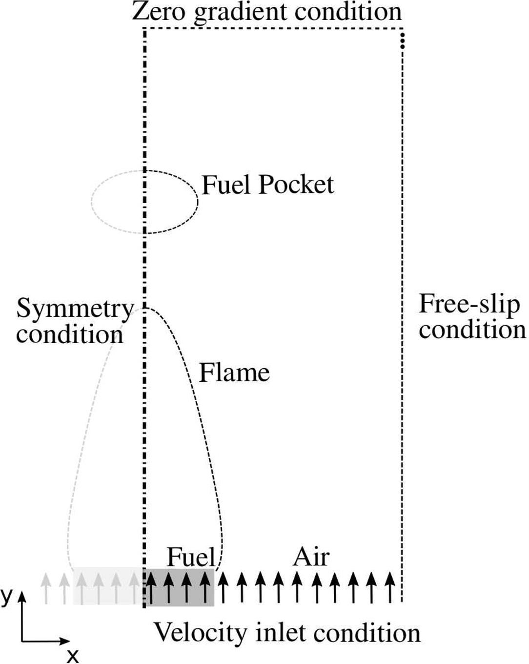
The unconfined flickering jet diffusion flame case was chosen to validate the full implementation of the present numerical code. The geometry of this case is 2D axisymmetric. As shown in Figure 12, the burner is composed by a fuel jet with a radius ![]() surrounded by a annular air stream with radius
surrounded by a annular air stream with radius ![]() . The fuel is methane diluted by
. The fuel is methane diluted by ![]() ,
, ![]() . The fuel and air burner inlet velocities are
. The fuel and air burner inlet velocities are ![]() and
and ![]() , respectively. The resulted Reynolds number, Péclet
number and Froude number for this case are
, respectively. The resulted Reynolds number, Péclet
number and Froude number for this case are ![]() ,
, ![]() , and
, and ![]() . Also, the Figure 12 shows the following boundary
conditions: on the top
. Also, the Figure 12 shows the following boundary
conditions: on the top ![]() and right
and right ![]() boundaries, free-slip condition is
imposed for velocities along with zero fluxes for the temperature, mixture
fraction and excess enthalpy. At the inlet section located at
boundaries, free-slip condition is
imposed for velocities along with zero fluxes for the temperature, mixture
fraction and excess enthalpy. At the inlet section located at ![]() , the velocity streamwise component is prescribed for
fuel and air, i.e.
, the velocity streamwise component is prescribed for
fuel and air, i.e. ![]() and
and ![]() , respectively. The mesh dependency tests showed no significant differences in the large-scale flame features, such as flicker frequency and points of fuel pocket detachment. The Courant–Friedrichs–Lewy condition was the base reference for the choice of the numerical parameters. For the present case, the CFL numbers for the physical and artificial-time integration, were chosen as CFLt=0.27 and CFLτ=0.2, respectively. Another key parameter of choice was the ability of the physical time-step to describe sufficiently well one cycle of flame flickering.
, respectively. The mesh dependency tests showed no significant differences in the large-scale flame features, such as flicker frequency and points of fuel pocket detachment. The Courant–Friedrichs–Lewy condition was the base reference for the choice of the numerical parameters. For the present case, the CFL numbers for the physical and artificial-time integration, were chosen as CFLt=0.27 and CFLτ=0.2, respectively. Another key parameter of choice was the ability of the physical time-step to describe sufficiently well one cycle of flame flickering.
The resulting times steps were ![]() and
and ![]() , for physical and artificial times, respectively. The value of β= 8 led to a suitable convergence rate for this set of time steps. The case introduced above reproduces the computations done by Davis et al. [28] who also used the flame sheet model, unit Lewis number hypothesis, and validated their results against the experimental data by Chen et al. [26]. One strong motivation behind the choice of this case was to assess the ability of the present code to describe the temporal behavior and the formation of vortical structures due to large density gradients and buoyancy effects. The low frequencies of flame oscillations (flame flickering) were in the range 5 Hz-15 Hz and independent of the fuel type, the geometry of the source of fuel and the flow field in the wake [25]. The coupling within the flow field between the accelerations around the flame and decelerations in the plume above it due to the buoyant force dramatically impacts the temperature and species field dynamics and is at the origin of the formation of large vortices outside of the flame. As a vortex ascends along the flame in direction of the tip, it is forced against the flame. Close to the flame tip, the vortex strangles the flame, a bottleneck appears featuring a large strain rate which leads to the local extinction of the flame ending up in the separation of part of the flame tip (fuel pockets) which is carried away by the flow [26].The frequency analysis of this behaviour of the flickering jet diffusion flame is shown in Figure 13.
, for physical and artificial times, respectively. The value of β= 8 led to a suitable convergence rate for this set of time steps. The case introduced above reproduces the computations done by Davis et al. [28] who also used the flame sheet model, unit Lewis number hypothesis, and validated their results against the experimental data by Chen et al. [26]. One strong motivation behind the choice of this case was to assess the ability of the present code to describe the temporal behavior and the formation of vortical structures due to large density gradients and buoyancy effects. The low frequencies of flame oscillations (flame flickering) were in the range 5 Hz-15 Hz and independent of the fuel type, the geometry of the source of fuel and the flow field in the wake [25]. The coupling within the flow field between the accelerations around the flame and decelerations in the plume above it due to the buoyant force dramatically impacts the temperature and species field dynamics and is at the origin of the formation of large vortices outside of the flame. As a vortex ascends along the flame in direction of the tip, it is forced against the flame. Close to the flame tip, the vortex strangles the flame, a bottleneck appears featuring a large strain rate which leads to the local extinction of the flame ending up in the separation of part of the flame tip (fuel pockets) which is carried away by the flow [26].The frequency analysis of this behaviour of the flickering jet diffusion flame is shown in Figure 13.
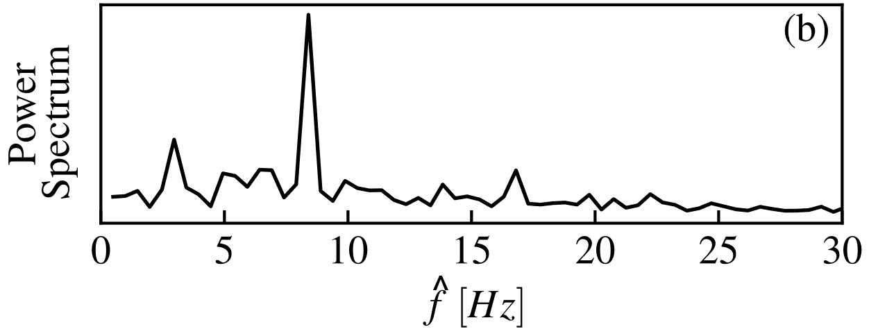
 , (b) power spectrum for the flame fluctuation.
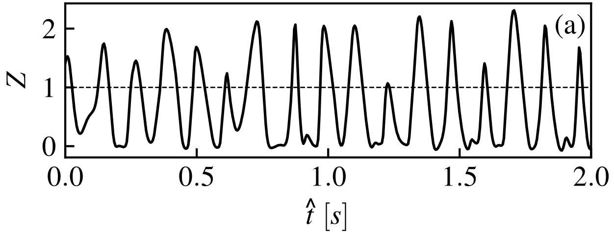
The mixture fraction history was chosen to represent the flame fluctuations at![]() , as shown in Figure 13a. The dashed line represents the stoichiometric value, thus, when the continuous line crosses this line, it means that the detachment of a hot pocket of fuel occurred. The power spectrum derived from the flame fluctuations are presented in Figure 13b. The numerically computed predominant frequency at the probe location of
, as shown in Figure 13a. The dashed line represents the stoichiometric value, thus, when the continuous line crosses this line, it means that the detachment of a hot pocket of fuel occurred. The power spectrum derived from the flame fluctuations are presented in Figure 13b. The numerically computed predominant frequency at the probe location of ![]()
![]() agrees well (relative error of 5.5%) with the value predicted by the correlation
agrees well (relative error of 5.5%) with the value predicted by the correlation ![]() ,
, ![]() , suggested by Sato et al. [27]. Since the large-scale instability is produced mainly by buoyancy, its frequency is an increasing function of the buoyancy strength as observed when plotting the Strouhal number as a function of the Froude number. The weaker secondary frequency peak visible in Figure 13b probably results from the preceding flame bulge interaction with the trailing one and is categorized here as a sub-harmonic. The flame evolution between
, suggested by Sato et al. [27]. Since the large-scale instability is produced mainly by buoyancy, its frequency is an increasing function of the buoyancy strength as observed when plotting the Strouhal number as a function of the Froude number. The weaker secondary frequency peak visible in Figure 13b probably results from the preceding flame bulge interaction with the trailing one and is categorized here as a sub-harmonic. The flame evolution between ![]() and
and ![]() is illustrated by Figure 14 which displays the temperatures isocontours and vorticity contours where the dimensional vorticity is defined by:
is illustrated by Figure 14 which displays the temperatures isocontours and vorticity contours where the dimensional vorticity is defined by:
 , (b)
, (b)  , (c)
, (c)  , (d)
, (d)  , (e)
, (e)  , (f)
, (f)  . The red isoline represents the flame sheet (Z=1) and the blue and the blue × marker represents the location of the probe from Figure 13a.
The bluish regions indicate the clockwise vortex structures and the reddish regions the counter clockwise vortex ones. The flame bulge is prominent by the isocontour of temperature. Meanwhile, the red isoline represents the flame sheet and evidences the detachment of fuel pockets. As previously described, these pockets are regions of hot gas enclosed by a flame that travels upward. The effective entrainment of oxidizer in the region of the axis of symmetry is found to be the main mechanism of the flame local extinction and release of this secondary flame. Detached fuel pockets can be observed in Figures 14c and 14f. Also, the Figure 14 displays the probe location where the data from Figure 13 were acquired. This location was chosen for illustrating the passage of the large vortical structure formed by the buoyant effect, a key feature for the correct flame flickering frequency analysis. Beyond the correct prediction of the flickering frequency, the unsteady flame structure appeared to be in line with the results presented in the literature (not shown here).
5. Conclusions
This work investigates the implementation of the unsteady artificial compressibility approach to simulate non-reacting and reacting flow fields in a zero Mach number framework. The resulting time-accurate scheme was tested in five different situations cases: the Stokes’ second problem, the unsteady wake flow past a circular cylinder, the flow around a heated cylinder placed in a square enclosure, a steady Tsuji diffusion flame, and a flickering buoyant diffusion flame. The flow over the oscillating plate and past a circular cylinder case were chosen to put into evidence the basic properties of the implemented time-accurate approach, such as the ability to describe unsteady non-reactive flows and its convergence rate. An analysis of the influence of the artificial compressibility factor on the convergence rate was carried out. As expected, the results showed that the stability of the numerical code is highly dependent on the value of the artificial compressibility factor and the computed number of time-steps required to reach convergence in artificial-time agreed very well with the expression presented by Chang and Kwak [6]. For the flow in the enclosure hosting a heated cylinder, a configuration that featured quite high density gradients, the predicted flow topology as well as the heat flux distribution along the enclosure walls matched very well those reported in the literature. Then, a comparison with experimental and numerical results was performed for a steady diffusion flame case. The simulated temperature profile and the flame shape were in good agreement with those reported in the literature, except in the region around the maximum temperature, where the reaction layer was not so well described, certainly because of the infinite-rate chemistry assumption considered here. The fifth case investigated the capability of the present approach to predict correctly the large scale unsteadiness of a flickering diffusion flame. An excellent agreement with the experimental results was observed in term of the fundamental frequency of the flame flickering. Qualitatively speaking, the predicted flame topology appeared to be in line with that observed experimentally.
Acknowledgments
Part of this work was done during a 1-year stay of the first author in France at Laboratoire de Mathématiques et de leurs Applications (CNRS/UPPA), Pau. Mariovane Donini gratefully acknowledges Coordenação de Aperfeiçoamento de Pessoal de Nível Superior – Brasil (CAPES) for its financial contribution to his research stay in France under grants numbers 88887.363086/2019-00 and 88882.444509/2019-01.
Nomenclature
References
[1] A. J. Chorin, “A numerical method for solving incompressible viscous flow problems,” Journal of Computational Physics, vol. 2, pp. 12–26, 1967. View Article
[2] P. Bruel, D. Karmed, and M. Champion, “A pseudo-compressibility method for reactive flows at zero Mach number,” International Journal of Computational Fluid Dynamics, vol. 7, no. 4, pp. 291–310, 1996. View Article
[3] W. Soh and J. W. Goodrich, “Unsteady solution of incompressible Navier-Stokes equations,” Journal of Computational Physics, vol. 79, no. 1, pp. 113–134, 1988. View Article
[4] S. Rogers and D. Kwak, “Numerical solution of the incompressible Navier-Stokes equations for steady-state and time-dependent problems,” in 27th Aerospace Sciences Meeting, 1989, p. 463. View Article
[5] C. Corvellec, P. Bruel, and V. Sabel’Nikov, “A time-accurate scheme for the calculations of unsteady reactive flows at low Mach number,”Journal for Numerical Methods in Fluids, vol. 29, no. 2, pp. 207–227, 1999. View Article
[6] J. Chang and D. Kwak, “On the method of pseudo-compressibility for numerically solving incompressible flows,” in 22nd Aerospace Sciences Meeting, 1984, p. 252. View Article
[7] W. M. Dourado, P. Bruel, and J. L. Azevedo, “A time-accurate pseudo-compressibility approach based on an unstructured hybrid finite volume technique applied to unsteady turbulent premixed flame propagation,” International Journal for Numerical Methods in Fluids, vol. 44, no. 10, pp. 1063–1091, 2004. View Article
[8] B. R. Hodges, “An artificial compressibility method for 1D simulation of open-channel and pressurized pipe flow,” Water, vol. 12, no. 6, pp. 1727, 2020. View Article
[9] E. S. Oran and J. P. Boris, Numerical simulation of reactive flow, New York, NY (United States); Cambridge University Press, 2001. View Article
[10] F. Bassi, F. Massa, L. Botti, and A. Colombo, “Artificial compressibility Godunov fluxes for variable density incompressible flows,” Computers and Fluids, vol. 169, pp. 186-200, 2018. View Article
[11] E Shapiro and D. Drikakis, “Artificial compressibility, characteristics-based schemes for variable density, incompressible, multi-species flows. Part I. Derivation of different formulations and constant density limit,” J ournal of Computational Physics, vol. 210, no. 2, pp. 584–607, 2005. View Article
[12] M. Fathi Azarkhavarani, B. Lessani, and S. Tabejamaat, “Artificial compressibility method on half-staggered grid for laminar radiative diffusion flames in axisymmetric coordinates,” Numerical Heat Transfer, Part B: Fundamentals, vol. 72, no. 5, pp. 392–407, 2017. View Article
[13] R. P. Bianchin, M. S. Donini, C. F. C. Cristaldo, and F. F. Fachini, “On the global structure and asymptotic stability of low-stretch diffusion flame: forced convection,” Proceedings of the Combustion Institute, vol. 37, pp. 1903–1910, 2019. View Article
[14] M S. Donini, C. F. Cristaldo, and F. F. Fachini, “Buoyant Tsuji diffusion flames: global flame structure and flow field,” Journal of Fluid Mechanics, vol. 895, pp. A17, 2020. View Article
[15] X. Xia and P. Zhang, “A vortex-dynamical scaling theory for flickering buoyant diffusion flames,” Journal of Fluid Mechanics, vol. 855, pp. 1156–1169, 2018. View Article
[16] M. Scha¨fer, S. Turek, F. Durst, E. Krause, and R. Rannacher, “Benchmark computations of laminar flow around a cylinder,” in Flow simulation with high-performance computers II. Springer, 1996, pp. 547–566. View Article
[17] H. Tsuji and I. Yamaoka, “The counterflow diffusion flame in the forward stagnation region of a porous cylinder,” Symposium (International) on Combustion, vol. 11, pp. 979–984, 1967. View Article
[18] H. Sclichting, Boundary layer theory. Mac Graw-Hill, 1979.
[19] A. Lin˜a´n and F. A. Williams, Fundamental aspects of combustion. New York, NY (United States);Oxford University Press, 1993.
[20] F. F. Fachini, A. Lin˜a´n, and F. A. Williams, “Theory of flame histories in droplet combustion at small stoichiometric fuel-air ratios,” AIAA Journal, vol. 37, pp. 1426–1435, 1999.
[21] F. F. Fachini, “Extended Shvab-Zel’dovich formulation for multicomponent-fuel diffusion flames,” International Journal of Heat and Mass Transfer , vol. 50, pp. 1035–1048, 2007. View Article
[22] B. S. Kim , D. S. Lee, M. Y. Ha and H. S. Yoon, “A numerical study of natural convection in a square enclosure with a circular cylinder at different vertical locations,” International Journal of Heat and Mass Transfer, vol. 51, no. 7-8, pp. 1888-1906, 2008. View Article
[23] S. S. Tsa and C. H. Chen, “Flame stabilization over a Tsuji burner by four-step chemical reaction,” Combustion Science and Technology, vol. 175, no. 11, pp. 2061–2093, 2003. View Article
[24] T. Dreier, B. Lange, J. Wolfrum, M. Zahn, F. Behrendt, and J. Warnatz, “Comparison of CARS measurements and calculations of the structure of laminar methane-air counterflow diffusion flames,” Berichte der Bunsengesellschaft fu¨r Physikalische Chemie, vol. 90, no. 11, pp. 1010–1015, 1986. View Article
[25] T.-Y. Toong, < R. F. Salant , J. M. Stopford , and G. Y. Anderson "Mechanisms of combustion instability," Symposium (International) on Combustion, vol. 10, no. 1, pp. 1301-1313. Elsevier, 1965. View Article
[26] L.-D. Chen , J. P.Seaba , W. M. Roquemore , and L. P. Goss , "Buoyant diffusion flames," Symposium (International) on Combustion, vol. 22. no. 1, pp. 677-684. Elsevier, 1989. View Article
[27] Sato, H., K. Amagai, and M. Arai. "Diffusion flames and their flickering motions related with Froude numbers under various gravity levels," Combustion and Flame, vol. 123, no.1-2, pp. 107-118, 2000. View Article
[28] R. W. Davis, E. F. Moore, L.-D. Chen, W. M. Roquemore, V. Vilimpoc and L. P. Goss, "A numerical/experimental study of the dynamic structure of a buoyant jet diffusion flame," Theoretical and Computational Fluid Dynamics , vol. 6, no. 2-3, pp. 113-123, 1994. View Article