Journal of Fluid Flow, Heat and Mass Transfer (JFFHMT)
ISSN: 2368-6111

Volume 8 - Year 2021 - Pages 60-71
DOI: 10.11159/jffhmt.2021.008
Film Thickness and Pressure Drop for Gas-Liquid Taylor Flow in Microchannels
Amin Etminan, Yuri S. Muzychka, Kevin Pope
Department of Mechanical Engineering, Faculty of Engineering and Applied Science
Memorial University of Newfoundland (MUN), St. John’s, NL, Canada A1A 3X5
aetminan@mun.ca; yurim@mun.ca; kpope@mun.ca
Abstract - This paper investigates the hydrodynamics of gas-liquid two-phase flow in an axisymmetric microchannel with a circular cross-sectional area. ANSYS Fluent was employed to simulate Taylor flow using the Volume of Fluid model to predict the interfacial phenomena between the two phases. Film thickness, bubble curvature, pressure drop, bubble/slug lengths are determined to investigate gas-liquid Taylor flow in micro capillaries. The results show that the liquid film thickness remains almost constant, but the length of the flat film region increases as the air bubble proceeds downstream. The predictions are validated with theoretical and experimental data in the literature, which show a good agreement.
Keywords: Computational Fluid Dynamics (CFD), Film Thickness, Microchannel, Taylor Flow, Transport Phenomena.
© Copyright 2021 Authors - This is an Open Access article published under the Creative Commons Attribution License terms Creative Commons Attribution License terms. Unrestricted use, distribution, and reproduction in any medium are permitted, provided the original work is properly cited.
Date Received: 2020-12-01
Date Accepted: 2020-12-04
Date Published: 2021-02-03
1. Introduction
Micro-structured mechanical systems are increasingly emerging in compact industrial applications. A microchannel has been designed to minimize pressure drop and maximize transport phenomena in numerous energy-related microfluidic purposes, such as heat exchangers, fuel cells, and microreactors. A typical gas-liquid two-phase flow refers to a mixture of two distinct phases and the phases are separated by interfacial lines. Such flows remain in the laminar flow regime due to predominant viscous and surface tension forces in them, which simplifies the numerical simulations by omitting the need for turbulence modelling.
The patterns of gas-liquid two-phase flows in microchannels are highly dependent on the transport phenomena, the type of channels, the phase’s superficial velocities, and the fluid properties, such as density, viscosity, and surface tension. Considering the remarkably low-velocity flow and very small-diameter channels, the gravitational and inertia forces are insignificant compared to surface tension and viscous forces. Various flow patterns, such as bubbly, Taylor, churn, annular, stratified, and wavy have been reported by investigators, e.g., [1]-[11]. An informative way to describe the patterns of multiphase flows is to map the flow pattern on an x-y graph, where the axes could be volumetric flow rate ratios, phase superficial velocities, and non-dimensional numbers such as Reynolds (Re), capillary (Ca), and Weber (We) [12]-[15]. Slug patterns occupies a large region in these maps. Consequently, accurate predictions of the gas bubble formation, growth, and propagation in microchannels are required, and calculations of some predominant flow parameters including void fraction, pressure drop, and liquid film thickness are taken into account.
In Taylor flow, the void fraction is defined as the fraction of the channel volume that is occupied by the gas phase. The value varies from 0 to 1 at different locations in the channel. The void fraction experiences fluctuations depending on the flow pattern, which is influenced by the volumetric flow rates and superficial velocities of phases. Therefore, the time-averaged void fraction is most often computed in two-phase flows. The most broadly used model to predict the void fraction in a wide variety of multiphase flows is the drift-flux model proposed by Zuber and Findlay [16]. In the model, the void fraction can be obtained as a function of the distribution parameter and gas volumetric flow rate, for a horizontal configuration, where the drift velocity is zero. Based on the type of multiphase flow, the configuration, and the flow pattern, different distribution parameters have been proposed, i.e., [1] and [17]-[21]. By assuming a long cylindrical gas bubble in a tube, Howard and Walsh [22] theoretically derived a distribution parameter in the drift-flux void fraction model. The void fraction and the pressure drop of gas-liquid flow in microchannels were measured by Kurimoto et al. [23]. Their data were compared to those provided by [24]-[26], resulting in a more reliable distribution parameter for predicting void fraction.
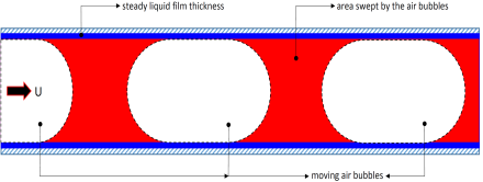
In Taylor flows, gas bubbles always are surrounded by a thin layer of continuous flow. Even though the thickness of the liquid is thin, it significantly affects the pressure drop, transport phenomena, and bubble curvature. As illustrated in Figure 1, the bubble’s curvatures follow a semi-hemispherical profiles, at both ends (the nose and tail caps). This type of curvature is well demonstrated in experimental and analytical data, e.g., [27]-[33]. A transition region that does not obey a semi hemispherical meniscus links the nose or tail cap with a flat/steady length of liquid film thickness.
Two other crucial parameters to characterize two-phase flows in the capillaries are the lengths of liquid slugs and gas bubbles. The lengths remained constant through the channels in a fully developed gas-liquid flow, which have been taken into account by investigators, such as [34]-[38].
Table 1 presents the non-dimensional lengths of a stable liquid slug and gas bubble in terms of a constant tube diameter. The deviation in the slug lengths gathered in Table 1 is due to flow conditions and tube configurations.
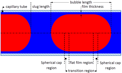
Table 1. Non-dimensional lengths of liquid slug and gas bubble.
| Author(s) |
Slug Length (Ls.D-1) |
Bubble Length (Lb.D-1) |
| Gupta et al., 2009 [39] | 1.3 | 2 |
| Qian et al., 2019 [40] | 2.13-3.25 | 1.54-1.97 |
| Qian et al., 2019 [40] | 2.07-3.02 | 1.56-2.06 |
This paper presents a numerical study of air/water flow in a microchannel. The gas bubble formation at a concentric junction is investigated to show how a gas bubble generates, propagates, and moves through the microchannel. The gas bubble profile, nose and tail curvatures, liquid film thickness, liquid slug lengths, gas bubble lengths, and steady or flat film thickness are predicted throughout the computational domain to capture interface and transport phenomena.
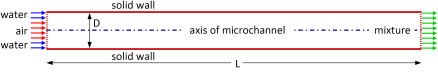
As illustrated in Figure 2, airflow enters at the core of the inlet cross-section and the water flow enters at an annular cross-section around the core. Air flow is in over 70% of the inlet diameter which means the same volumetric flow rates for both flows in an axisymmetric microchannel. A mixture of phases exits the channel at the outlet.
2. Governing Equations and Mathematical Model
An incompressible gas-liquid two-phase flow is assumed in a two-dimensional microchannel where each phase is a Newtonian fluid with constant thermophysical properties. The gas and liquid phases are immiscible and phase change does not occur within the microchannel. Therefore, the continuity and the momentum equations take on the following forms

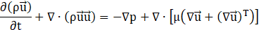

where μ and ρ denote the dynamic viscosity and density, respectively. The last term in the momentum equation represents the surface tension force per unit area, which is approximately considered as a body force surrounding the interface line between phases [41],

where σ, κ, δ, and ![]() represent the surface tension force, radius of curvature or surface normal (viewed from the gas bubble), Dirac delta function, and unit normal vector on the interfacial line (from the gas to liquid phases), respectively.
represent the surface tension force, radius of curvature or surface normal (viewed from the gas bubble), Dirac delta function, and unit normal vector on the interfacial line (from the gas to liquid phases), respectively.
The curvature of the interface line and normal vector are defined as functions of the volume fraction (α):


The gravitational force ![]() becomes negligible when there are both a small-diameter microchannel and dominant surface tension effects, which appear in Eötvös number (Eo),
becomes negligible when there are both a small-diameter microchannel and dominant surface tension effects, which appear in Eötvös number (Eo),
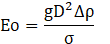
where D, g, and Δρ represent the microchannel diameter, gravitational acceleration, and difference between phase densities, respectively. Eo is estimated to be on the order of 10-2, therefore, the gravitational term is neglected in the momentum equation [13]. Different criteria has been developed to justify the dominant surface tension compared to the gravitational force, such as Eo≪(2π)2 proposed by Brauner and Moalem-Maron [42].
The momentum equation solution predicts a shared velocity field for both phases, throughout the computational domain. The accuracy of the predicted velocities, in the vicinity of the interface, can be adversely affected when the difference between superficial velocities is significant. Due to the presence of two phases in the computational domain, a volume fraction equation can be assumed,
The value of the volume fraction varies from 0 to 1. In Taylor flow, where a train of the gas bubbles moves in a continuous liquid flow, the importance of the volume fraction becomes insignificant inside the gas bubbles and within the liquid slugs. This parameter must be taken into account in the vicinity of the gas-liquid interface region to accurately predict the interfacial effects and momentum transport between phases.
To capture the gas-liquid interface in multiphase flows, ANSYS Fluent offers the Level Set and the Volume of Fluid (VoF) methods. The Level Set method assumes a value of zero as the level set of a smooth function at the interface of the two phases. The amount of the level set function is negative in the gas phase and positive in the liquid phase. The VoF method solves a single set of momentum equations and calculates the volume fraction equation of each phase within the computational domain. This approach can be used for steady and transient two-phase flows to identify the gas-liquid interface. A user-defined source term can be specified on the right side of the volume fraction equation, which ANSYS Fluent assumes to be zero by default. The volume-fraction weighted average is employed to compute the thermophysical properties of the two phases, such as density and viscosity in the governing equations. If the volume fraction of the second phase (α2) is tracked, then the amount of property (φ) in each control volume in the two-phase flow is represented by
where the subscripts 1 and 2 denote each phase. One limitation is that the solution may not converge for viscosity ratios greater than 103. In an arbitrary fluid volume, three cases are possible:αi=0 when the volume is empty of fluid ith, αi=1 when the volume is full of fluid ith, and 0<αi<1 when the volume contains the interface between phases 1 and 2.
An explicit approach is selected to discretize time steps by a standard finite-difference interpolation scheme applied to the volume fractions at the previous time step. In particular, ANSYS Fluent can compute the values of the face fluxes near the interface line by interpolation either using an interface reconstruction or a Finite Volume (FV) discretization scheme. The reconstruction scheme obtains the amount of flux on the faces whenever a cell is filled with a phase. The finite volume discretization approach can only be employed with an explicit VoF method using first-order upwind or second-order upwind, and QUICK algorithms. The VoF method calculates a time step based on the transient time characteristic over a control volume, which is not necessarily equal in other governing equations. In the vicinity of the interface region, the ratio of the volume of each cell and the sum of the outgoing flux from the faces of the finite volume leads to the time taken to empty a cell. The Courant number (Co) includes the smallest such time-step,
where the Δx and Ufluid represent the grid size and fluid velocity, respectively. In the following simulations, the maximum value of the Co is 0.25, and a fixed time step of 10-6 is employed to reduce total computational time unless it causes an unexpected increase in the Courant number. To prevent divergence of the solution in such cases, a variable time step between 10-6 and 10-7 is selected, particularly at the moments of gas bubble breakup.
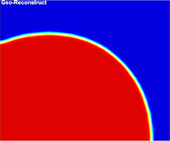
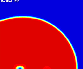
Conversely, the implicit approach does not have limitations on the Courant number enabling larger grid sizes and time-steps compared to the explicit approach. However, its higher numerical diffusion in the interface region reduces the accuracy of predictions for interface curvature between phases. The explicit approach allows employing a Geo-Reconstruct as the volume fraction discretization scheme resulting in a clear and crisp prediction of interface curvature with no numerical diffusion. The Modified HRIC creates a thicker interface, a longer air bubble, and considerable numerical diffusion on the axis inside the bubble. This weakness causes divergence during air bubble breakup. Consequently, the explicit approach along with the Geo-Reconstruct discretization scheme are maintained for the simulations in this paper.
Surface tension effects appear due to the interaction and attractive forces between molecules in the flow. Surface tension acts inward at the surface and is required to stay in equilibrium. The pressure gradient creates an outward force to balance surface tension force at the surface. In ANSYS Fluent, the surface tension force is modeled as a continuum surface force [41]. In that model, a wall-adhesion angle (θw ) or a contact angle in conjunction with the surface tension force needs to be specified. Therefore, the surface normal vector is represented by

where ![]() and
and ![]() are the unit vectors normal and tangential to the wall. The contact angle must be specified. Some other researchers assumed dry-out on walls showing no liquid film thickness and the gas bubbles were in direct contact with the walls, e.g., [43] and [44]. Conversely, significant mesh refinement near the walls is required to predict boundary layer behaviour and liquid film thickness which was employed by Qian and Lawal [37].
are the unit vectors normal and tangential to the wall. The contact angle must be specified. Some other researchers assumed dry-out on walls showing no liquid film thickness and the gas bubbles were in direct contact with the walls, e.g., [43] and [44]. Conversely, significant mesh refinement near the walls is required to predict boundary layer behaviour and liquid film thickness which was employed by Qian and Lawal [37].
 (a)
(a)
 (b)
(b)
(air is coloured red and water is coloured blue)
3. Problem Description
This study is carried out to perform a systematic numerical simulation of two-phase flow in a two-dimensional microchannel. The geometric parameters of the microchannel are depicted in Figure 2 where the channel diameter (D) is 0.5 mm and the channel length (L) is 5 mm. The entrance length of channels is 10 times the diameter [53], therefore, the flow is developing. The velocity inlet boundary condition is assumed for both phases. Outlet flow boundary condition is applied at the exit plane of the channel. The axisymmetric geometry of the microchannel allows the simulations to be conducted for only half of the actual computational domain resulting in lower computational time. Therefore, the axis boundary condition is set on the axis of the channel, where the normal gradients for all variables are zero. Finally, the typical no-slip boundary condition is presumed at the solid wall of the microchannel. The properties of operating fluid flows are at room temperature of 25°C (Table 2). The superficial velocities of the air and water are 0.245 m.s-1 and 0.255 m.s-1, respectively, and the average velocities of phases is 0.5 m.s-1. These flow conditions result in Ca, Re, and We values of 0.00618, 279.93, and 1.73, respectively. Air and water flows enter the channel uniformly when the channel is filled with water at an average velocity as the initial condition for the simulations.
Table 2. Thermophysical properties of air and water used in the simulations.
| Fluid |
Density
(kg.m-3) |
Dynamic Viscosity (kg.m-1.s-1) |
Surface Tension
(N.m-1) |
| Air | 1.1845 | 1.849×10⁻⁵ | 0.072 |
| Water | 997.1 | 8.905×10⁻⁴ |
4. Numerical Formulation
To avoid a de-coupling of velocity and pressure variables for Scale-Resolving Simulations (SRS), a proper algorithm must be chosen considering a few key factors: geometry of the problem, properties of fluids involved, flow regime, and activated additional models (if any). The uncomplicated geometry and non-activated additional models for the laminar flow regime limit the convergence criterion by the pressure-velocity coupling. Semi-Implicit Method for Pressure Linked Equations-Consistent (SIMPLEC) algorithm can be used to couple pressure and velocity fields in the Navier-Stokes equations. The SIMPLEC is designed to manipulate the proper corrections in the velocity equation by removing less significant terms (e.g., [45]-[47]). The rectangular computational domain, constructed from square cells, and the absence of distorted meshes allows the skewness correction to be set to 0, which significantly reduces the convergence difficulties in the simulations, [48]. The SIMPLEC algorithm computes the gradients of scalar flow parameters, such as pressure, density, volume fraction, and velocity components at the centre of cells using the values of the parameters at the cell faces. The pressure-based algorithm employs under-relaxation factors to control the values of variables at every iteration. Thus, the pressure and momentum under-relaxation factors are set to 0.3 and 0.7, respectively, to improve convergence speed and solution stability. The scaled residuals show a slightly decreasing trend as the time is marching forward and remain on the order of 10-6 to 10-7. For time-dependent flows, ANSYS can discretize the generic transport equations by iterative and Non-Iterative Time Advancement (NITA) schemes. In the present study, a first order non-iterative time marching scheme is employed to reduce the computational time for each time-step. The NITA scheme does not require the outer iterations resulting in a significant reduction of computational expense ([48]-[50]). This scheme is also beneficial for the user-defined quantity of sub-iterations for each individual governing equation, as well as the correction tolerance which are set to 10-7.
Least Squares cell-based, Green-Gauss cell-based, and Green-Gauss node-based approaches are available to calculate not only the gradient interpolation of the flow parameters, but also secondary diffusion terms and the derivatives of velocity at the centre of cell faces. An accurate method, which provides the highest accuracy, and least computational expense is highly problem-dependent ([39] and [48]). The incompressibility of the flow in the present study allows the Least Square to be selected. For pressure interpolation, the PRESTO! scheme is not appropriate because of its high dissipation rate resulting in a delay ([45] and [47]). The Body Force Weighted, Second-Order Upwind, and Geo-Reconstruct schemes are assumed for pressure, momentum, and volume fraction interpolations, respectively, to achieve high accuracy predictions with minimal computational expense. The second-order upwind scheme discretizes the convective terms using two upstream nodes to calculate variables at the cell faces. Its accuracy is second-order regarding Taylor series analysis, [48]. Another scheme for momentum interpolation is QUICK which stands for Quadratic Upstream Interpolation for Convective Kinematics. The QUICK discretizes the momentum equation and computes a higher-order value of convective variables at the cell faces. This is using a second-order central difference for diffusion terms and a third-order central difference for convection terms. This scheme is of benefit to a weighted average of second-order upwind to interpolate scalar variables at the cell faces. The QUICK scheme provides more accuracy compared to second-order upwind for computing variables on structured meshes ([45] and [47]). Hence, the QUICK discretization scheme has been employed in the following simulations. In addition to an appropriate time step and the number of iterations for each time step, under relaxation factor adjustment is required to make a robust solver and prevent divergence. A poor-quality mesh can make numerical instabilities during solutions. Therefore, a comprehensive mesh study has been carried out to find an independent grid size.
5. Grid Independence Study
Proper grid resolution is important in numerical studies to capture transport phenomena, particularly Taylor flow in microchannels. The film thickness is computed by different empirical correlations, e.g., [27], [29], [31], [33], [51], and [54]. The film thickness ranges from 9 to 13 microns, which will be used to establish the grid size. Most of the correlations are based on experimental data of air/water two-phase flows except [51]. The liquid film thickness is typically measured in a fully developed Taylor flow where the measuring location is far from the junction and the film thickness remains constant. Whereas, this study is investigating developing Taylor flow in the entrance region of a microchannel.
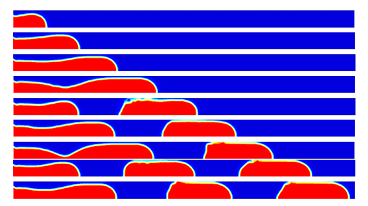
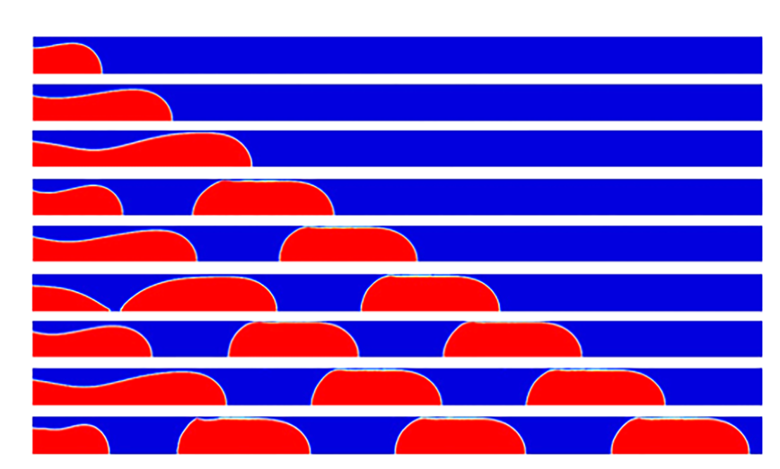
Three discretization approaches can be considered; coarse, fine-coarse, and fine. The coarse approach divides the whole domain into square-shaped cells starting with 25×25 μm cells as the first trial. Figure 4 represents the liquid volume fraction for a coarse-size mesh of 25 microns (case I) at every 1 ms to show the air-bubbles emerging and moving downstream. Since the size of cells is greater than the approximate film thickness, the boundary layer, liquid film, and interfacial near the wall cannot be properly predicted. The boundary layer is not realized by the simulations and dry-out is observed at the wall. Furthermore, the air/water interface becomes thick, sharp, and without a semi hemispherical curvature at the rear end.
Four other refinements are investigated to determine an independent mesh which are presented in Table 3, at 9 ms. Case I is not able to capture film thickness and only two bubbles are generated over 9 ms. By halving the grid size, case II, three shorter air bubbles are observed, but the liquid film thickness is not properly predicted. Case III captures liquid film thickness successfully and three bullet shape air bubbles are generated over 9 ms, when the lengths of bubbles are decreased with time marching. As illustrated in Figure 5, for a coarse-sized mesh of 6.25 μm, at every 1 ms, further decreasing the grid size, predicts an approximately identical flow pattern. The grid refinement from case III to IV makes a 3.7% variation, while from case IV to V leads to a 1.4% variation. The flow patterns, lengths and quantity of slugs and plugs are not dependent on the mesh refinement further than case IV. Therefore, the following numerical predictions are conducted with the mesh refinement of case IV.
(air is coloured red and water is coloured blue)
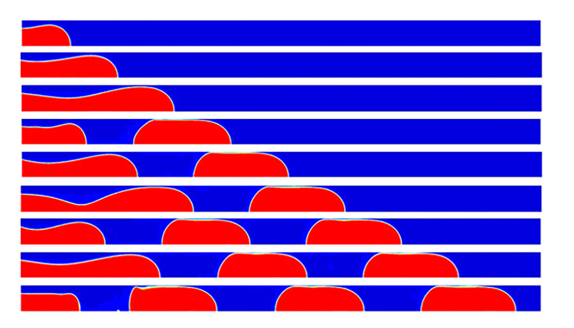
A time history of air bubble formation, growing, necking, breaking off, and moving through the channel is illustrated in Figure 5 for mesh case IV. The semi hemispherical nose meniscus remains constant, but the tail meniscus is deforming from an approximate flat cap to semi hemispherical as the bubble moves downstream. The liquid film thickness is captured throughout the channel. The liquid film thickness involves only two grids and it is not sufficient to capture the boundary layer and transport phenomena properly. Consequently, mesh refinement over a thickness of 15 μm along the channel’s wall is required to find an adequate size of grids which estimates the thickness accurately and prevents non-physical pressure jumps across the interface [39].
(air is coloured red and water is coloured blue)
Table 3. Mesh independence for core region.
| Case | Mesh Size (μm) | Bubble Breakup (ms) | Film Thickness (μm) | Slug Length (Ls.D-1) | Bubble Length (Lb.D-1) | |||||
| 3rd | 2nd | 1st | 2nd | 1st | 3rd | 2nd | 1st | |||
| I | 25 | ----- | 7.04 | 4.23 | fully dry-out | ----- | 1.32 | ----- | 2.11 | 1.89 |
| II | 12.5 | 8.84 | 6.08 | 3.74 | partially dry-out | 1.22 | 1.16 | 1.72 | 1.74 | 1.91 |
| III | 8.33 | 8.78 | 6.29 | 3.62 | 10.41 | 1.14 | 1.12 | 1.70 | 1.72 | 1.84 |
| IV | 6.25 | 8.45 | 6.10 | 3.57 | 10.24 | 1.12 | 1.09 | 1.68 | 1.71 | 1.82 |
| V | 5 | 8.43 | 6.08 | 3.52 | 10.23 | 1.12 | 1.10 | 1.67 | 1.71 | 1.81 |
Table 4. Mesh independence for near the wall region.
| Case | Mesh Size (μm) | Film Thickness (μm) | Slug Length (Ls.D-1) | Bubble Length (Lb.D-1) | |||||
| 3rd | 2nd | 1st | 2nd | 1st | 3rd | 2nd | 1st | ||
| I | 3 | 12.50 | 11.50 | 11.00 | 1.15 | 1.14 | 1.79 | 1.76 | 1.85 |
| II | 2.5 | 10.75 | 11.14 | 10.94 | 1.16 | 1.14 | 1.78 | 1.75 | 1.85 |
| III | 2.43 | 10.62 | 11.10 | 10.83 | 1.16 | 1.13 | 1.78 | 1.75 | 1.86 |
In the fine-coarse approach, the presence of the solid walls encourages the mesh generation process to employ a non-uniform distribution perpendicular to the flow direction. Over a thickness of 15 μm along with the channel’s wall, 5, 6, and 7 cells are considered to enable the simulations of capturing boundary layer and film thickness successfully. The length of cells is set to a constant value of 6.25 μm. The fine grid sizes near the wall and the coarse grid in the core region of the microchannel allows accurate predictions of film thickness and also reduces the computational time. The corresponding total numbers of cells are 34,400, 35,200, and 36,000. With these meshes, a linear slope of the interface line between two phases at the inlet can be assumed to calculate the advection of each phase at the cell faces. The refinements have resulted in the average film thicknesses of 11.67, 10.94, and 10.85 μm for mesh sizes of 3, 2.5, and 2.43 μm, respectively (see Table 4). Since an insignificant change of 0.8% is predicted by mesh refining from 2.5 to 2.43 μm, the grid size of 2.5 μm is selected. This mesh refinement prevents non-physical pressure jump in uniform liquid film region as observed by Gupta et al. [39] and results in minimum false diffusion and truncation error ([45] and [47]).
As illustrated in Figure 6, the interface line between phases occupies the entire computational domain as the air bubbles move downstream. It means that mesh refinement should be applied over the domain entirely with equal-sized cells in both directions. A square-shape mesh of 2.5 μm is utilized to determine possible changes in the flow pattern and the quantitative aspects of problem. The results show non-remarkable deviations and therefore, the third approach is not a proper mesh generation approach. Therefore, a square coarse grid can be adopted throughout the core region and a refined grid near the wall of the channel for the modelling of gas-liquid two-phase flow.
The computational domain is discretized into 35,200 cells and the simulations run on a DELL workstation with Intel® Xeon® E5-1650 v3 @3.5 GHz processor. CPU cash and memory (RAM) are 15 MB and 32 GB, respectively. The average time-marching for a time-step calculation is 2.87 seconds and each simulation takes approximately 7 hours to complete.
Figure 7 shows a time history of volume fraction for a non-uniform fine-sized mesh, case II, at every 1 ms. A train of air bubbles (coloured red) follows a hydrodynamics evolution process involving emersion, elongation, filling, necking, breaking off, and moving. The bullet-like bubbles travel downstream with an insignificant change in the nose curvature, while the rear curvature experiences an undulation over one millisecond after breakup moment. According to Table 4, maximum variations of 5%, 1.7%, and 3.6% are observed for bubble length, slug length, and film thickness, respectively.
(air is coloured red and water is coloured blue)
6. Results and Discussion
A developing Taylor flow causes some ripples at the liquid film which are shown by the enlarged views of the film regions of three air bubbles in Figure 8. The ripples disappear as the bubble moves downstream, due to time marching.
The length of the flat film region becomes longer (the nose and tail transition lengths become shorter) as the bubble travels to the outlet, as presented in Table 5. The variations of the lengths of transition and flat regions become smaller as the bubble moves. The semi hemispherical meniscus at the nose and rear parts of the bubbles can be approximately fitted by two spheres at the nose and tail with a radius of R1 and R2, respectively. As is also presented in Table 5, the radius of the nose curvature is less than that of the tail but the bullet-like profile of the second bubble remains almost constant.
As illustrated in Figure 9, the highest axial velocity is at the centre of the bubbles along the axis of the microchannel. At the caps of the bubbles, the axial velocity component is lower and the radial velocity component is higher at the bubble’s centre increased. This behaviour was previously found by Gupta et al. [39]
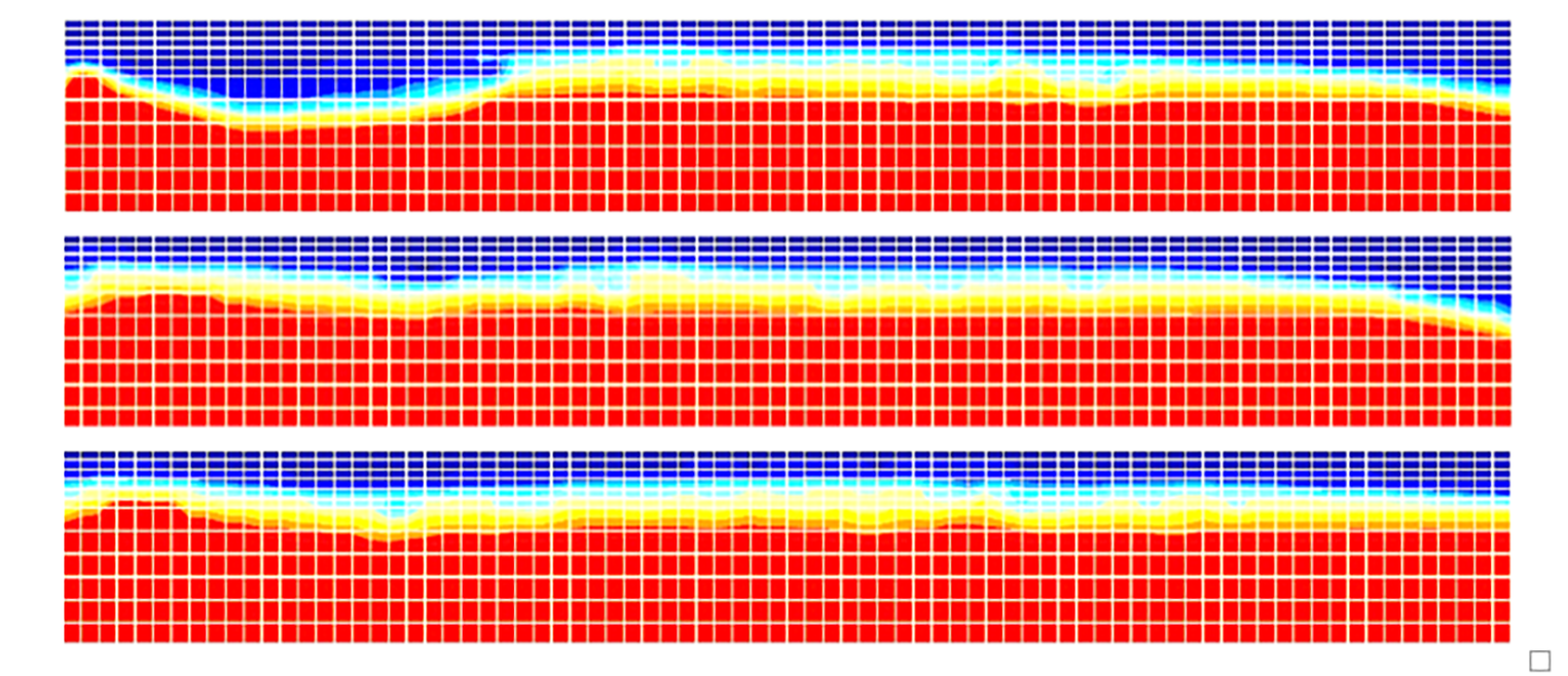
Table 5. Predicted air bubble shapes and geometric details.
| Bubble |
Meniscus Radius
(μm) |
Transition Length
(μm) |
Flat Region
Length
(μm) |
||
| R1 | R2 | nose | tail | ||
| 1st | 210 | 240 | 120 | 109 | 502 |
| 2nd | 210 | 240 | 166 | 158 | 399 |
| 3rd | 200 | 240 | 227 | 275 | 265 |
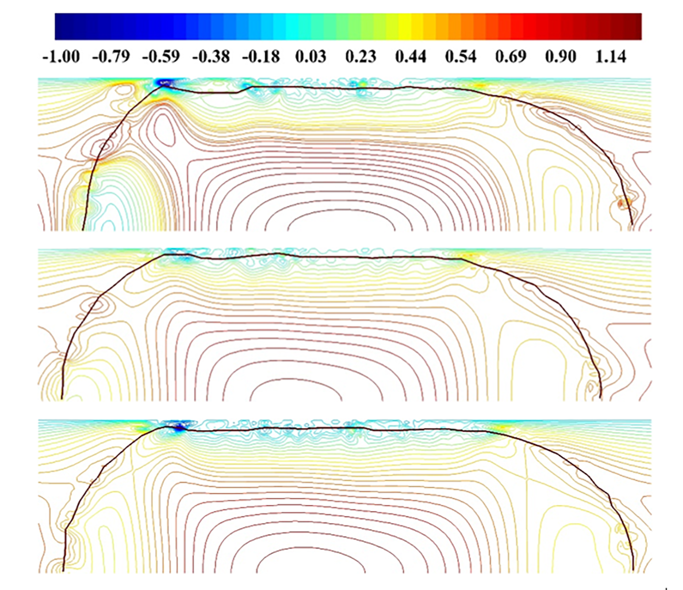
(thick solid line indicates the curvature of the bubbles)
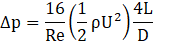
Two homogenous and separated flow models have been employed by researchers to predict the frictional pressure drop. The first model postulates the same velocity for both gas and liquid phases, which implies that the slip ratio at the interactive boundaries is equal to one. This model considers two or more different phases as a single phase. The values of the flow properties are dependent on the quality, while the frictional pressure drop can be computed by single-phase flow theory derived by White [53] as follows:
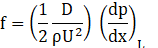
where D, L, U, and x indicates the diameter of the tube, the length, the mean velocity (UGS+ULS ), and the axial direction of the channel. The Hagen-Poiseuille equation is a physical law to compute the pressure drop of a Newtonian and incompressible flow through a long and circular tube with a constant cross-section area. The flow regime remained laminar due to the Reynolds number of the microflows, where the friction factor becomes f=16/Re for round tubes and the Eq. (11) can be rearranged in the following way.
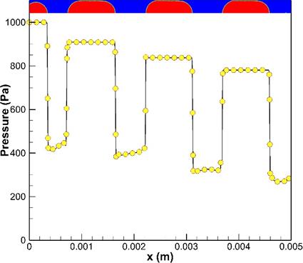
In Taylor flow, the pressure drop is affected by the curvatures of the slugs, the slug and plug lengths, and steady film thickness. Figure 10, shows the pressure distribution on the axis of the microchannel for gas-liquid Taylor flow and at 9 ms. A volume fraction plot has been affixed to this figure where the dispersed phase is coloured red and the continuous phase is coloured blue.
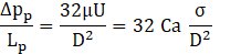
The pressure drop over a unit cell can also be described by three components, which has been proposed by [3], [5], and [54]:

where the last two terms in Eq. (13) represent the total pressure drop over the gas bubble. The pressure drop over the liquid plug can be calculated by Hagen-Poiseuille Eq. (12) in fully developed flow without internal circulation as below:
According to Eq. (14), the pressure drop over the liquid plug is 56,955 Pa/m where the corresponding value from the present numerical simulation over two halves of adjacent liquid plugs to the first bubble is 60,345 Pa/m indicating an acceptable agreement with 5% deviation. The difference becomes much more for the second unit cell where the flow regime is slightly further away from fully developed conditions. As illustrated in Figure 10, the pressure distributions over the steady film region are almost constant and ∆pf is negligible, which agrees with Fouilland et al. [5]. Conversely, the normal stress at the interface within the steady film region is no longer present and the Laplace pressure at the interface can predict the pressure difference. The pressure difference between inside the gas bubble and the liquid at the wall is σ/Rb=301 Pa, which the corresponding value from the simulation for the first unit cell is so close with less than 2% deviation. As the pressure distribution at the wall, within the flat film region, shows fluctuations due to the interactions between the wall and interface (not displayed here), its mean value is computed by integrating over the flat region. However, the interfacial pressure difference in the hemispherical nose region of the first air bubble is of the order of 2σ/Rb=602 Pa, whereas the simulations predict 513 Pa. The difference is due to the developing conditions and the assumption of non-exact hemispherical shape of the gas bubble. The last term in Eq. (13) can be calculated by lubrication theory discussed by Bretherton [27] assuming insignificant inertia forces and exact semi-hemispherical profile at both caps of the bubble.
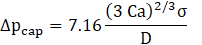
The numerically predicted bubble cap pressure difference is ⁓61 Pa compared to 72 Pa predicted by Eq. (15). This deviation can also be attributed to the significant difference between the nose and the rear meniscus, non-exact semi hemispherical cap curvatures, and the inertia effects. Consequently, the pressure drop per a unit length is 60,700 Pa.
7. Conclusions
In this paper, numerical predictions of air/water Taylor flow, for developing flow, in a microchannel with a circular cross-sectional area were investigated. A mesh independence study showed that the mesh size caused different interactions between two phases and the channel wall, i.e., dry-out, partially dry-out, and fully wetted to explain whether the wall was kept dry or wet. The new numerical predictions showed that the liquid film thickness of the bubbles remained almost constant, but the length of the flat film region increased as the air bubble moved downstream. The results of this paper provide useful new insights into gas-liquid Taylor flow.
Acknowledgment
We would like to thank the Natural Sciences and Engineering Research Council of Canada (NSERC) for financial support under grant numbers 200439 and 209780.
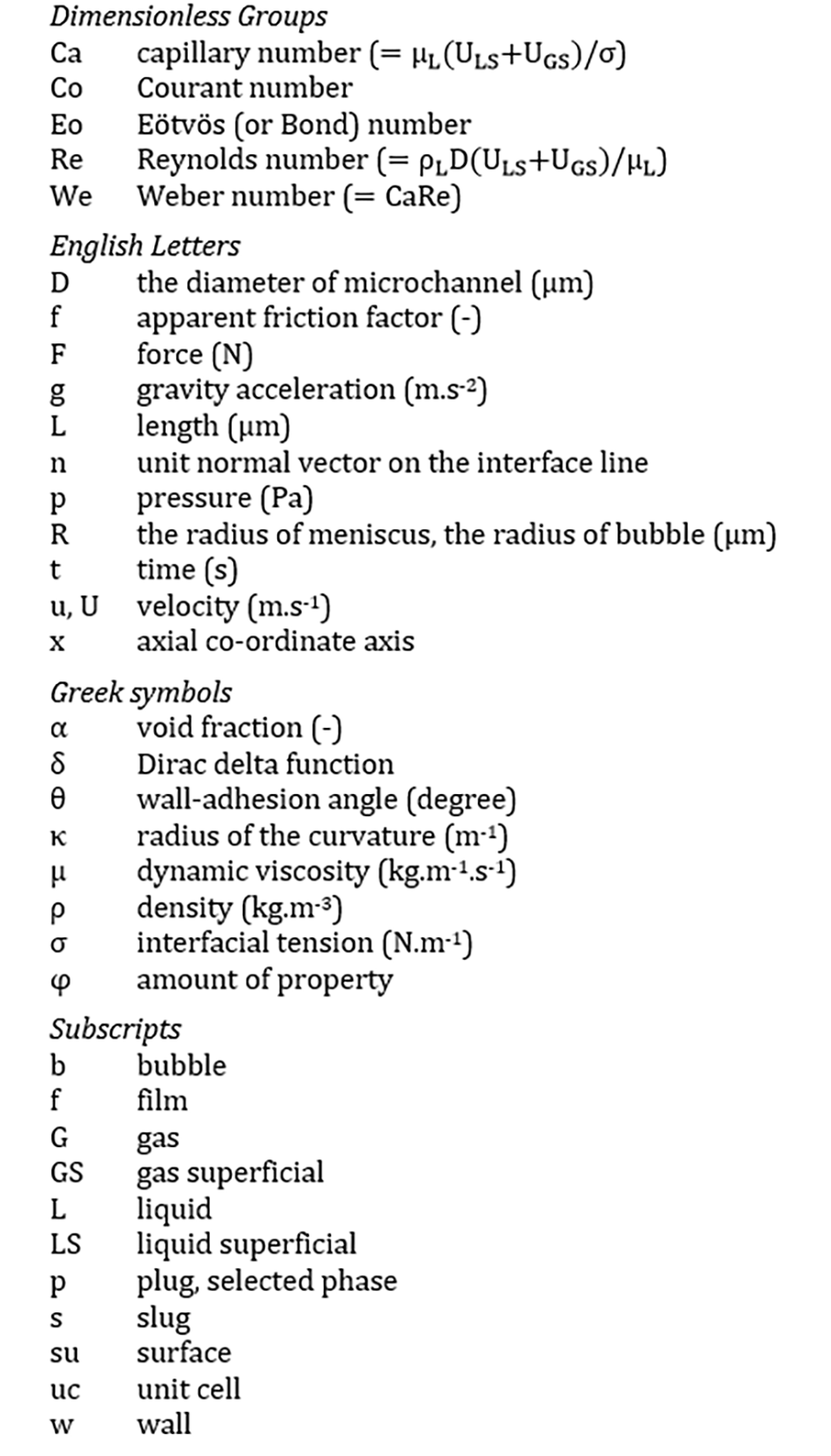
Nomenclature
References
[1] A. Kawahara, M. Sadatomi, K. Nei and H. Matsuo, “Experimental study on bubble velocity, void fraction and pressure drop for gas-liquid two-phase flow in a circular microchannel,” International Journal of Heat and Fluid Flow, vol. 30, pp. 831–841, 2009. View Article
[2] T. Cubaud and C.M. Ho, “Transport of bubbles in square microchannels,” Physics of Fluids, vol. 16(12), pp. 4575–4585, 2004. View Article
[3] M.T. Kreutzer, F. Kapteijn, J.A. Moulijn, C.R. Kleijn and J.J. Heiszwolf, “Inertial and interfacial effects on pressure drop of Taylor flow in capillaries,” American Institute of Chemical Engineers, vol. 51(9), pp. 2428–2440, 2005a. View Article
[4] J. Yue, L. Luo, Y. Gonthier, G. Chen and Q. Yuan, “An experimental investigation of gas-liquid two-phase flow in single microchannel contactors,” Chemical Engineering Science, vol. 63(16), pp. 4189–4202, 2008. View Article
[5] T.S. Fouilland, D.F. Fletcher and B.S. Haynes, “Film and slug behaviour in intermittent slug-annular microchannel flows,” Chemical Engineering Science, vol. 65(19), pp. 5344–355, 2010. View Article
[6] M.N. Kashid, A. Renken and L. Kiwi-Minsker, “Influence of flow regime on mass transfer in different types of microchannels,” Industrial & Engineering Chemistry Research, vol. 50(11), pp. 6906–6914, 2011. View Article
[7] A. Sur and D. Liu, “Adiabatic air-water two-phase flow in circular microchannels,” International Journal of Thermal Sciences, vol. 53, pp. 18–34, 2012. View Article
[8] J.M. Bolivar and B. Nidetzky, “Multiphase biotransformations in microstructured reactors: opportunities for biocatalytic process intensification and smart flow processing,” Green Processing and Synthesis, vol. 2(6), pp. 541–559, 2013. View Article
[9] A.A. Yagodnitsyna, A.V. Kovalev and A.V. Bilsky, “Flow patterns of immiscible liquid-liquid flow in a rectangular microchannel with T-junction,” Chemical Engineering Journal, vol. 303, pp. 547–554, 2016. View Article
[10] R. Kong, S. Kim, S. Bajorek, K. Tien and C. Hoxie, “Effects of pipe size on horizontal two-phase flow: Flow regimes, pressure drop, two-phase flow parameters, and drift-flux analysis,” Experimental Thermal and Fluid Science, vol. 96, pp. 75–89, 2018. View Article
[11] Deendarlianto, A. Rahmandhika, A. Widyatama, O. Dinaryanto, A. Widyaparaga and Indarto, “Experimental study on the hydrodynamic behavior of gas-liquid air-water two-phase flow near the transition to slug flow in horizontal pipes,” International Journal of Heat and Mass Transfer , vol. 130, pp. 187–203, 2019. View Article
[12] S.S. Jayawardena, V. Balakotaiah and L.C. Witte, “Flow Pattern Transition Maps for Microgravity Two-Phase Flows,” AIChE Journal, vol. 43(6 ), pp. 1637–1640, 1997. View Article
[13] K.A. Triplett, S.M. Ghiaasiaan, S.I. Abdel-Khalik and D.L. Sadowskia, “Gas-liquid two-phase flow in microchannels Part I: two-phase flow patterns,” International Journal of Multiphase Flow, vol. 25(3), pp. 377–394, 1999. View Article
[14] P.M.-Y. Chung and M. Kawaji, “The effect of channel diameter on adiabatic two-phase flow characteristics in microchannels,” International Journal of Multiphase Flow, vol. 30(7–8), pp. 735–761, 2004. View Article
[15] S.M. Ghiaasiaan, Two Phase Flow, “Boiling and Condensation in Conventional and Miniature Systems,” Cambridge University Press, New York, 2014.
[16] N. Zuber and J.A. Findlay, “Average Volumetric Concentration in Two-Phase Flow Systems,” Journal of Heat Transfer, vol. 87(4), pp. 453–468, 1968. View Article
[17] A. Kariyasaki, T. Fukano, A. Ousaka and M. Kagawa, “Isothermal Air-Water Two-Phase Up-and Downward flows in a Vertical Capillary Tube: 1st Report, Flow Pattern and Void Fraction,” Transactions of the Japan Society of Mechanical Engineers Series B , vol. 58(553), pp. 2684–2690, 1992 (in Japanese). View Article
[18] K. Mishima and T. Hibiki, “Some characteristics of air-water two-phase flow in small diameter vertical tubes,” International Journal of Multiphase Flow, vol. 22(4), pp. 703–712, 1996. View Article
[19] S. Saisorn and S. Wongwises, “Flow pattern, void fraction and pressure drop of two-phase air-water flow in a horizontal circular micro-channel,” Experimental Thermal and Fluid Science, vol. 32(3), pp. 748–760, 2008. View Article
[20] M. Ishii and T. Hibiki, “Thermo-Fluid Dynamics of Two-Phase Flow,” Springer-Verlag, New York, 2011. View Article
[21] H. Minagawa, H. Asama and T. Yasuda, “Void fraction and frictional pressure drop of gas-liquid slug flow in a microtube,” Transactions of the Japan Society of Mechanical Engineers Series B , vol. 79(804), pp. 1500–1513, 2013 (in Japanese). View Article
[22] J.A. Howard and P.A. Walsh, Review and extensions to film thickness and relative bubble drift velocity prediction methods in laminar Taylor or slug flows. International Journal of Multiphase Flow, vol. 55, pp. 32–44, 2013. View Article
[23] R. Kurimoto, K. Nakazawa, H. Minagawa and T. Yasuda, “Prediction models of void fraction and pressure drop for gas-liquid slug flow in microchannels,” Experimental Thermal and Fluid Science , vol. 88 , pp. 124–133, 2017. View Article
[24] K. Hayashi, R. Kurimoto and A. Tomiyama, “Dimensional analysis of terminal velocity of Taylor bubble in a vertical pipe,” Multiphase Science and Technology, vol. 22(3), pp. 197–210, 2010. View Article
[25] K. Hayashi, R. Kurimoto and A. Tomiyama, “Terminal velocity of a Taylor drop in a vertical pipe,” International Journal of Multiphase Flow, vol. 37(3), pp. 241–251, 2011. View Article
[26] R. Kurimoto, K. Hayashi and A. Tomiyama, “Terminal velocities of clean and fully contaminated drops in vertical pipes,” International Journal of Multiphase Flow, vol. 49, pp. 8–23, 2013. View Article
[27] F.P. Bretherton, “The motion of long bubbles in tubes,” Journal of Fluid Mechanics, vol. 10(2), pp. 166–188, 1961. View Article
[28] G.I. Taylor, “Deposition of a viscous fluid on the wall of a tube,” Journal of Fluid Mechanics, vol. 10(2), pp. 161–165, 1961. View Article
[29] L.W. Schwartz, H.M. Princen and A.D. Kiss, “On the motion of bubbles in capillary tubes,” Journal of Fluid Mechanics, vol. 172, pp. 259–275, 1986. View Article
[30] S. Irandoust and B. Andersson, “Simulation of flow and mass transfer in Taylor flow through a capillary,” Computers & Chemical Engineering, vol. 13(4–5), pp. 519–526, 1989. View Article
[31] P. Aussillous and D. Quéré, “Quick deposition of a fluid on the wall of a Tube,” Physics of Fluids, vol. 12(10), pp. 2367–2371, 2000. View Article
[32] H. Fujioka and J.B. Grotberg, “The steady propagation of a surfactant-laden liquid plug in a two dimensional channel,” Physics of Fluids, vol. 17, pp. 082102, 2005. View Article
[33] Y. Han and N. Shikazono, “Measurement of the liquid film thickness in micro tube slug flow,” International Journal of Heat and Fluid Flow, vol. 30(5), pp. 842–853, 2009. View Article
[34] S. Laborie, C. Cabassud, L. Durand-Bourlier and J.M. Lainé, “Characterisation of gas-liquid two-phase flow inside capillaries,” Chemical Engineering Science, vol. 54(23), pp. 5723–5735, 1999. View Article
[35] R.R. Broekhuis, R.M. Machado and A.F. Nordquist, “The ejector-driven monolith loop reactor experiments and modelling,” Catalysis Today, vol. 69(1–4), pp. 93–97, 2001. View Article
[36] P. Garstecki, M. Fuerstman, H. Stone and G. Whitesides, “Formation of droplets and bubbles in a microfluidic T-junction-scaling and mechanism of break-up,” Lab on a Chip, vol. 6(3), pp. 437–446, 2006. View Article
[37] D. Qian and A. Lawal, “Numerical study on gas and liquid slugs for Taylor flow in a T-junction microchannel,” Chemical Engineering Science, vol. 61(23), pp. 7609, 2006. View Article
[38] Y. Song, F. Xin, G. Guangyong, S. Lou, C. Cao and J. Wang, “Uniform generation of water slugs in air flowing through superhydrophobic microchannels with T-junction,” Chemical Engineering Science, vol. 199, pp. 439–450, 2019. View Article
[39] R. Gupta, D.F. Fletcher and B.S. Haynes, “On the CFD modelling of Taylor flow in microchannels,” Chemical Engineering Science, vol. 64(12), pp. 2941–2950, 2009. View Article
[40] J.Y. Qian, M.R. Chen, Z. Wu, Z.J. Jin and B. Sunden, “Effects of a Dynamic Injection Flow Rate on Slug Generation in a Cross-Junction Square Microchannel,” Processes, vol. 7(10), pp. 765, 2019. View Article
[41] J.U. Brackbill, D.B. Kothe and C. Zemach, “A continuum method for modeling surface tension,” Journal of Computational Physics, vol. 100(2), pp. 335–354, 1992. View Article
[42] N. Brauner and D. Moalem-Maron, “Identification of the range of small diameter conduits, regarding two-phase flow pattern transition,” International Communications in Heat and Mass Transfer, vol. 19(1), pp. 29–39, 1992. View Article
[43] Q. He, K. Fukagata and N. Kasagi, “Numerical simulation of gas-liquid two-phase flow and heat transfer with dry-out in a micro tube,” In: Proceedings: Sixth International Conference on Multiphase Flow , Leipzig, Germany, 2007. View Article
[44] V. Kumar, S. Vashisth, Y. Hoarau and K.D.P. Nigam, “Slug flow in curved microreactors: hydrodynamic study,” Chemical Engineering Science, vol. 62 (24), pp. 7494–7504, 2007. View Article
[45] S.V. Patankar, “Numerical Heat Transfer and Fluid Flow,” Taylor & Francis; 1st edition, 1980.
[46] J.P. van Doormaal and G.D. Raithby, “Enhancement of SIMPLE method for predicting incompressible fluid flows,” Numerical Heat Transfer, vol. 7(2), pp. 147–63, 1984. View Article
[47] H.K. Versteeg and W. Malalasekera, “An Introduction to Computational Fluid Dynamics: the finite volume method,” 2nd ed., Harlow, Eng.; Toronto: Pearson/Prentice Hall, 2007.
[48] ANSYS Fluent 18.1.0 Users' Guide, SAS Inc., 2017.
[49] S. Armsfield and R. Street, “The Fractional-Step Method for the Navier-Stokes Equations on Staggered Grids: Accuracy of Three Variations,” Journal of Computational Physics, vol. 153(2), pp. 660–665, 1999. View Article
[50] J.B. Perot, “An Analysis of the Fractional Step Method,” Journal of Computational Physics, vol. 108(1), pp. 51–58, 1993. View Article
[51] M.T. Kreutzer, P. Du, J.J. Heiszwolf, F. Kapteijn and J.A. Moulijn, “Mass transfer characteristics of three–phase monolith reactors,” Chemical Engineering Science , vol. 56(21–22), pp. 6015–6023, 2001. View Article
[52] K. Fukagata, N. Kasagi, P. Ua-arayaporn and T. Himeno, “Numerical simulation of gas-liquid two-phase flow and convective heat transfer in a micro tube,” International Journal of Heat and Fluid Flow, vol. 28(1), pp. 72–82, 2007. View Article
[53] F.M. White, “Fluid Mechanics,” McGraw–Hill, 2011.
[54] D. Ni, F.J. Hong, P. Cheng and G. Chen, “Numerical study of liquid-gas and liquid-liquid Taylor flows using a two-phase flow model based on Arbitrary-Lagrangian-Eulerian (ALE) Formulation,” International Communications in Heat and Mass Transfer, vol. 88, pp. 37–47, 2017. View Article