Journal of Fluid Flow, Heat and Mass Transfer (JFFHMT)
ISSN: 2368-6111

Volume 5 - Year 2018 - Pages 32-43
DOI: 10.11159/jffhmt.2018.004
Heat Transfer Investigation in an Engine ExhaustType Pulsating Flow
Marco Simonetti1, Christian Caillol1, Pascal Higelin1, Clément Dumand2, Emmanuel Revol2
1Laboratoire PRISME, Université d’Orléans
8 rue Léonard de Vinci, 45072 Orléans Cedex 2, France
marco.simonetti@univ-orleans.fr
2Groupe PSA
Route de Gizy, Vélizy-Villacoublay, France
Abstract - In many practical engineering situations, such as in the exhaust pipes of Internal Combustion Engines, heat is transferred under conditions of pulsating flow. In these conditions, the heat transfer mechanism is affected by the pulsating flow parameters. The objective of the present work was to experimentally investigate heat transfers for pulsatile turbulent flows in a pipe. A specific experimental apparatus able to reproduce a pulsating flow representative of the engine exhaust was designed. A stationary turbulent hot air flow with a Reynolds number ranging from 1.8x10⁴ to 3.5x10⁴, based on the time averaged velocity, is excited through a pulsating mechanism and exchanges thermal energy with a steel pipe. Pulsation frequency ranges from 10 to 95 Hz. The effects of pulsation frequency and pipe length on the convective heat transfer were evaluated. It was observed that flow pulsation enhances convective heat transfers in comparison with the steady case. The results highlight that, when the flow is excited with a pulsation frequency equal to a resonance mode of the system, a local maximum of the heat transfer rate appears. This behaviour was found to be independent of the pipe length. Instantaneous measurements of air velocity and temperature demonstrated that the increase in the energy axial advection due to the oscillating component of the velocity is the major cause of the heat transfer enhancement.
Keywords: Convective Heat Transfer Enhancement, Pulsating Flow, Internal Combustion Engine, Waste Heat Recovery.
© Copyright 2018 Authors - This is an Open Access article published under the Creative Commons Attribution License terms Creative Commons Attribution License terms. Unrestricted use, distribution, and reproduction in any medium are permitted, provided the original work is properly cited.
Date Received: 2017-12-04
Date Accepted: 2018-04-03
Date Published: 2018-06-18
1. Introduction
Legislation on vehicle emissions continues to become ever more stringent in an effort to minimize the impact of Internal Combustion Engines (ICEs) on the environment, constraining engine manufacturers to face the challenge of increasing engine efficiency and decreasing pollutant emissions. ICE efficiency is still improving but it is today limited at best to around 40%, as a large part of the energy contained in the fuel is lost in coolant, oil, exhaust gas and air around the engine. Considering the exergetic limits, Waste Energy Recovery (WER) is a promising way to go further in fuel saving and pollutant emission control: a waste heat recovery system produces power by using the heat energy available at the exhaust, without additional fuel input. Besides the use of WER to increase ICE efficiency, particular attention is also being paid to the design of catalytic converters and exhaust manifold to comply with emission standards requirements. In order to reduce emission during the cold start phase, various solutions can be implemented in both the engine and exhaust system, such as a faster catalytic converter action to increase the efficiency of exhaust gas processing. Among all the techniques proposed in the past few years, as demonstrated by the work of Petković et al. [1], passive systems are being widely investigated. They include a simple constructional alteration on the exhaust manifold, which can be used to reduce heat losses to the atmosphere. For WER systems as well as for the design of engine exhausts, good management of the heat transfer phenomena is an important requirement, as demonstrated by the work of Host et al. [2]. Heat transfers in engine manifolds occur under pulsating conditions. The term ‘pulsating’ is used for cycle-stationary flows in which the oscillations occur around a time-averaged value different from zero. Although for a stationary flow the Reynolds number characterizes the laminar or turbulent behaviour of the bulk flow, the amplitude and the frequency of the superimposed oscillations play a dominant role in the structures of the pulsating flow. In recent decades, extensive studies have been dedicated to pulsating flows, and their associated heat transfer process, in a wide range of experimental configurations. However, some available results are contradictory and the main questions are still open: does pulsation enhance or else degrade heat transfers compared to a steady flow? What are the main heat transfer mechanisms?
2. Related Work
Dec et al. [3], [4] studied the influence of pulsation frequency (f), amplitude and mean flow rate on the heat transfers for a pulse combustor tail pipe. Pulsation frequency was varied from 67 to 100 Hz, for a Reynolds number (Re) based on the time-averaged velocity varying between 3100 and 4750. Several mechanisms responsible for the heat transfer enhancement in reversing, oscillating turbulent flows were presented and discussed, among which acoustic streaming, entrance effects and the turbulence intensity increase. According to the authors, the influence of both acoustic streaming (which corresponds to the appearance of a secondary time-averaged velocity component having the form of large longitudinal recirculation cells) and entrance effects on the observed Nusselt number (Nu) enhancement was small. In further studies, time-resolved velocities [5] and temperatures [6] were analysed to describe the heat transfer enhancement mechanism. The results suggested that a combination of increased shear-layer generated turbulence and strong convection at the zero-velocity crossings by transverse flows was the most plausible explanation for the mechanism causing the observed heat transfer enhancement. Xu et al. [7] studied the flow properties of a self-excited Helmholtz pulse combustor elbow tailpipe. The results showed that, due to pulsation and flow reversal, Dean Vortex forming, shedding and reforming process periodically contribute to convective heat transfer enhancement. With the same type of experimental apparatus, Zhai et al. [8] proposed a Nusselt correlation for the pulsating flow, based on the addition of two independent physical properties. Applying the quasi-steady theory and the Vaschy-Buckingham theorem to the convection heat transfer problem, the ratio between the velocity amplitude and the time-averaged velocity and the ratio between the pulsation velocity scale and the time-averaged velocity were found to be the aforementioned independent physical properties. Several studies were also conducted on turbulent and laminar pulsating pipe flows. In the work of Patel et al. [9], the Reynolds number ranged from 7000 to 16500, while the pulsation frequency was varied from 1 Hz to 3.33 Hz. Results showed that the Nusselt number was strongly affected by both pulsation frequency and Reynolds number with a 44.4% maximum enhancement of the heat transfer coefficient at the pulsation frequency of 3.33 Hz. In a study on a pulsating turbulent water stream, Zohir [10] also pointed out that the heat transfer coefficient was strongly affected by pulsation frequency and amplitude and by the Reynolds number. The improvement in heat transfers was attributed to an increased level of turbulence and the introduction of forced convection in the boundary layer. In the study by Li et al. [11] on heat transfer in turbulent pulsating pipe flows, the time-averaged Reynolds number varied from 6×10⁴ to 12×104 and pulsation frequency ranged from 0 to 100 Hz. Results showed that the Nusselt number was improved with the increase in the Reynolds number and the pulsation amplitude, defined as the ratio between the pressure amplitudes at the inlet and outlet of the pipe. Otherwise, the Nusselt number decreased with the increase in the Womersley number (Wo) up to a value of Wo=130, but a maximum value was obtained for a pulsation frequency of 90Hz approximately, corresponding to Wo=150. Habib et al. [12] studied the heat transfers in laminar pulsating pipe flows, where the Reynolds number and the pulsation frequency ranged from 780 to 1987, and from 1 to 29.5 Hz respectively. The results showed that the pulsation frequency affected heat transfers stronger than the Reynolds number. Compared to a steady flow, both an enhancement and a reduction of heat transfers, corresponding to different pulsation frequency ranges, were observed. In turbulent conditions (for a Reynolds numbers range of 5000 – 29000), Habib et al. [13] also found an increase or a decrease of heat transfer as a function of the pulsation frequency. The turbulent bursting mode was identified as a possible explanation for the observed heat transfer modification. Likewise, in the work of Monschandreou et al. [14], both an enhancement and a degradation of heat transfers was observed: the results indicated that, in a range of moderate frequency values, the effect of the pulsation was to increase the bulk temperature of the fluid and the Nusselt number, but the effect was reversed outside this range. The experimental studies by Said et al. [15] and Nishandar et al. [16] confirmed that the heat transfer coefficient was either increased or decreased function of the pulsation frequency in turbulent conditions. Elshafei et al. [17] studied numerically conducted a numerical study of the heat transfers for a fully developed pulsating turbulent flow over a range of 104 ≤ Re ≤ 4×10⁴ and 0 ≤ ƒ ≤ 70 Hz and the results were compared with the available experimental data. Results showed a slight reduction in the time-averaged Nusselt number with respect to that of a steady flow. However, in the fully developed established region, the local Nusselt number was either increased or decreased, compared to Nu values for steady flow, depending on the frequency parameter. As reported by the aforementioned surveys, it has been frequently observed that pulsation frequency may have an impact on the convective heat transfers. However, the variety of the experimental configurations and the variety of the pulsation creation mechanisms have led to some controversies: both enhancement and degradation of convective heat transfers have been observed. Besides, the main physical mechanisms involved have not been fully described. In the present study, an experimental investigation was conducted on heat transfer phenomena for a pulsating turbulent pipe flow, in a wide range of variation of the physical parameters. The main purposes were to investigate the impact of the pulsation frequency on heat transfers and to identify the main physical mechanisms involved in the heat transfer modification. Particular attention was paid to the calculation of the time-averaged convective heat transfer by developing an analytical formulation of the heat transfer problem. The design of an experimental apparatus, able to reproduce a pulsating pipe hot air flow over a range of 10 ≤ ƒ ≤ 95 Hz and 1.8×10⁴ ≤ Re ≤ 3.5×10⁴, representative of engine exhaust flow operating conditions, is presented. In the test-rig, the pulsating hot air flow exchanges thermal energy with cold water flowing in the opposite direction. The work presented in this paper focuses only on the time- and space-averaged characterization of the convective heat transfers, using a 1D flow hypothesis. Data collection and reduction are presented; results are reported and discussed based on this assumption.
3. Experimental Setup and Procedures
3. 1. Experimental Setup
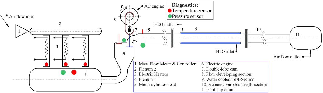
A schematic diagram of the pulsatile flow facility is depicted in figure 1. It comprises three main parts: the first one produces a hot stationary air flow, the second one transforms the stationary flow to a pulsating flow, and in the last part, in which the flow develops, heat transfers are estimated. In the first part of the test rig, the dry compressed air mass flow rate is measured and regulated by a Brooks SLA5853S {1}, a thermal effect mass flow meter with a maximum flow rate of 2500 Nl/min and with a calibration uncertainty of 0.73% of full scale. Then, air is heated by three Sylvania inline air heaters {3} with a total electric power of 12 kW, ensuring a maximum air temperature of 400°C at the maximum mass flow rate. Hot flow is finally stored in a 30-litre steel tank {4} designed to withstand a maximum air pressure of 10 bar and to dampen the flow pulsation coming back from the pulse generator. Once the hot air flow has been generated it is forced to pass through the pulsating mechanism {5-7}: a mono-cylinder head was chosen to produce a pulsating flow with a maximum frequency of 95 Hz, equipped with a classical pushrod valve train entrained by an electric engine with a power of 3 kW and a nominal velocity of 3000 rpm. In detail, hot air flows from the bottom of the cylinder head and only one of the two intake valves is alternately closed and opened to create the pulsating flow. The intake valve was chosen because of its higher diameter. Air leakages in the cylinder head were experimentally estimated to be below 0.5 kg/h, leading to an error on the mass flow rate measurement of <1%. In order to determine the camshaft position and rotation velocity, an encoder with a resolution of 0.1° is placed on the camshaft. Once the pulsating flow is generated, it is forced to pass through a steel pipe {8-10} in which it develops and exchanges thermal energy. Finally, at the end of the pipe, a 6-litre tank {11} is placed to muffle pressure pulsations. The entire flow facility is then linked to the exhaust line of the laboratory. As shown in figure 1, the steel pipe is composed of three different sections: the first one, called developing section {8}, has a length of 2.65 meters and a pipe length/internal diameter ratio of 48.4. It was designed to be long enough to completely develop the velocity flow field in the case of a steady turbulent flow.
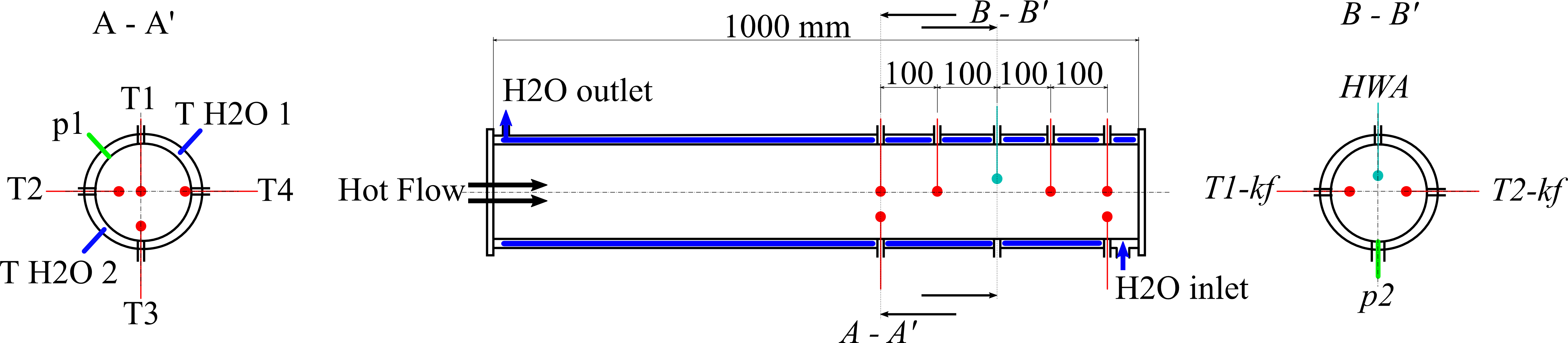
The pipe is thermally insulated to avoid high heat energy losses. The test section {9} (detailed in figure 2), with a length of 1 meter, is placed at the outlet of the developing section and is designed to be able to characterize heat transfers.
The test section consists of a double-wall
pipe, in which the pulsating air and cold water flow in opposite directions,
respectively in the internal and external parts of the pipe. Water cooling has
the advantage of making it possible to manage the wall temperature and of
having a homogeneous temperature field in the internal wall of the pipe. Inlet
and outlet water temperatures are measured by two 0.5 mm sheathed K-type
thermocouples in order to evaluate the total time-averaged convective heat
transfer ![]() (see Eq. 7). A Kistler
Type 2621F conditioning unit, with a maximum cooling power up to 1500 Watt, is
used to provide a maximum water flow rate of 6.1 l/min. As shown in figure 2,
at a distance from the beginning of the test-section of 10 times the internal
pipe diameter, several sensors are placed to measure the air velocity,
temperature and pressure. In particular, in order to calculate the air bulk
temperature, which corresponds to the integral of temperature on the cross
section, in the first measuring section (A – A’ in figure 2) four sheathed K-type
thermocouples with a 0.5 mm diameter are placed at different distances from the
wall, respectively 1, 0.5, 0.125 and 0.0625 times the pipe radius. Furthermore,
a Kulite pressure transducer is placed to measure the instantaneous static
pressure of air. The same measuring configuration was used for the outlet
section of the test-section. For the remaining sections, except the section B –
B’, only one 0.5 mm sheathed K-type thermocouple is placed at the centreline of
the pipe. In the section B – B’, in addition to a Kulite pressure transducer, a
Constant Temperature Anemometer and two unsheathed micro-thermocouples are
placed to measure the instantaneous radial profiles of air velocity and
temperature. In particular, a Dantec 55P71 double wire probe (HWA in figure 2) was
used to measure the air velocity magnitude and to detect flow reversal. The
energy balance equation applied to the hot junction of a thermocouple describes
the temperature difference between the gas and the hot junction with a
thermocouple temperature delay due to the finite mass of the hot junction and
due to the convective heat transfer between the fluid and the thermocouple.
Assuming negligible thermal conduction and radiation in this equation, the hot
junction temperature can be modelled as a first-order system, where the time
constant represents the requested time the sensor needs to reach the gas
temperature. For rapid temperature measurements, such time constant has to be
compared to the dynamic of the flow properties variation in order to know if a
compensation of the time delay has to be applied to the thermocouple signal to
compute the real fluid temperature. A Kalman Filter method [18] was applied to the signal of the two
micro-thermocouples (T1-kf, T2-kf in figure 2) to calculate in-situ the time
constant of the sensor in order to correct the raw thermocouple measurements
and to estimate the actual air temperature. The method has been experimentally
validated using a reference temperature signal measured
with a cold wire with a diameter of 1 µm which has a frequency bandwidth up to
1 kHz. An uncertainty less than 3% has been found. The
HWA and the micro-thermocouples are connected to the pipe with a concentric
screw system with a thread pitch of 1 mm. As shown in figure 1, downstream the
test-section, a pipe with a variable length was used. The total length of the
pipe can vary from 3.61 meters to 5.91 meters. A NI-9035 cRIO and the LabView
software were used to control all the devices in the experimental apparatus and
to acquire data.
(see Eq. 7). A Kistler
Type 2621F conditioning unit, with a maximum cooling power up to 1500 Watt, is
used to provide a maximum water flow rate of 6.1 l/min. As shown in figure 2,
at a distance from the beginning of the test-section of 10 times the internal
pipe diameter, several sensors are placed to measure the air velocity,
temperature and pressure. In particular, in order to calculate the air bulk
temperature, which corresponds to the integral of temperature on the cross
section, in the first measuring section (A – A’ in figure 2) four sheathed K-type
thermocouples with a 0.5 mm diameter are placed at different distances from the
wall, respectively 1, 0.5, 0.125 and 0.0625 times the pipe radius. Furthermore,
a Kulite pressure transducer is placed to measure the instantaneous static
pressure of air. The same measuring configuration was used for the outlet
section of the test-section. For the remaining sections, except the section B –
B’, only one 0.5 mm sheathed K-type thermocouple is placed at the centreline of
the pipe. In the section B – B’, in addition to a Kulite pressure transducer, a
Constant Temperature Anemometer and two unsheathed micro-thermocouples are
placed to measure the instantaneous radial profiles of air velocity and
temperature. In particular, a Dantec 55P71 double wire probe (HWA in figure 2) was
used to measure the air velocity magnitude and to detect flow reversal. The
energy balance equation applied to the hot junction of a thermocouple describes
the temperature difference between the gas and the hot junction with a
thermocouple temperature delay due to the finite mass of the hot junction and
due to the convective heat transfer between the fluid and the thermocouple.
Assuming negligible thermal conduction and radiation in this equation, the hot
junction temperature can be modelled as a first-order system, where the time
constant represents the requested time the sensor needs to reach the gas
temperature. For rapid temperature measurements, such time constant has to be
compared to the dynamic of the flow properties variation in order to know if a
compensation of the time delay has to be applied to the thermocouple signal to
compute the real fluid temperature. A Kalman Filter method [18] was applied to the signal of the two
micro-thermocouples (T1-kf, T2-kf in figure 2) to calculate in-situ the time
constant of the sensor in order to correct the raw thermocouple measurements
and to estimate the actual air temperature. The method has been experimentally
validated using a reference temperature signal measured
with a cold wire with a diameter of 1 µm which has a frequency bandwidth up to
1 kHz. An uncertainty less than 3% has been found. The
HWA and the micro-thermocouples are connected to the pipe with a concentric
screw system with a thread pitch of 1 mm. As shown in figure 1, downstream the
test-section, a pipe with a variable length was used. The total length of the
pipe can vary from 3.61 meters to 5.91 meters. A NI-9035 cRIO and the LabView
software were used to control all the devices in the experimental apparatus and
to acquire data.
3. 2. Procedure
The study of the impact of the flow pulsation on heat transfer phenomena is achieved by exciting a steady hot air flow with a pulsation frequency ranging from 0 to 95 Hz. The minimum attainable frequency is 10 Hz; for lower frequencies the electric motor is unable to perform constant speed revolution. A time-averaged mass flow rate varies from 90 to 130 kg/h and is forced to flow through the mono-cylinder head. The centreline air temperature at the inlet of the test-section is maintained constant at 150°C for all experiments by regulating the electric power of the air heaters with a PID controller. These flow conditions correspond to a time-averaged Reynolds number varying from 19000 to 35000, corresponding to turbulent flow state conditions.
The cooling water temperature at the inlet of the test-section is kept constant at 17.4°C for each experiment, with a maximum test-by-test variation of around 0.2°C.
The instantaneous mass flow rate profile imposed on the flow, in this manner, is dependent on the flow pulsation frequency and the pipe acoustic responses. This means that while the time-averaged component of the mass flow rate is kept constant for all the flow pulsations, the oscillating component is not constant. In order to extract coherent phenomena responsible for the convective heat transfer mechanisms, three different pipe lengths were investigated (3.69, 4.69 and 5.91 meters). In this manner both the flow pulsation frequency and the acoustic resonance modes of the pipe were varied, making it possible to study the influence of one characteristic on the other.
To characterize the acoustic resonance modes of the test-rig pipe for all the different lengths, a further experiment was conducted: after a thermal stabilisation of the experimental apparatus, by generating a steady hot air flow with an air temperature of 150°C at the inlet of the test section, the system was subjected to a pressure impulse and then allowed to resonate. Instantaneous pressures were measured at four different axial positions along the pipe and analysed to compute the resonance mode frequencies of the system.
4. Analytical Formulation of the Problem
As previously mentioned, the effect of the pulsation on heat transfers can be characterized in terms of the relative Nusselt number 𝑁𝑢𝑟el, defined as the ratio of the time-averaged Nusselt number for the pulsating flow to the corresponding one for a steady flow with the same time-averaged Reynolds number. For a cylindrical control volume, the time-averaged Nusselt number is defined as in the following equation:

where: ![]() is the time-averaged
convective heat transfer,
is the time-averaged
convective heat transfer, ![]() the internal diameter of
the pipe,
the internal diameter of
the pipe, ![]() the exchange surface,
the exchange surface, ![]() the logarithmic mean
temperature difference between the air and the internal wall of the pipe and
the logarithmic mean
temperature difference between the air and the internal wall of the pipe and ![]() the thermal conductivity of air.
the thermal conductivity of air.
The relative Nusselt number definition has
been adopted in several previous studies because of its ability to bring out
the impact of the pulsation frequency on heat transfers and to identify a
corrective coefficient for a Nusselt correlation accounting for pulsating
effects. The practical difficulty in such an approach consists in correctly assessing
the time-averaged convective heat transfer![]() Since in some applications the measurement of the heat flux exchanged with a
solid wall is difficult to achieve,
Since in some applications the measurement of the heat flux exchanged with a
solid wall is difficult to achieve, ![]() is computed starting from
the air flow properties by solving the energy balance equation.
is computed starting from
the air flow properties by solving the energy balance equation.
The time-averaged convective heat transfer
is generally computed from the variation of the time-averaged component of the
air enthalpy through the inlet and outlet sections of the control volume, but
it is shown in the following development that this calculation does not take
into account characteristic terms related to the pulsating component of the
flow. In the present work, ![]() is derived from the time-averaged and space-integrated form of the instantaneous energy
balance equation for a pulsating turbulent pipe flow. The terms related to the
heat flux propagated from the advection of the oscillating component of the
flow are highlighted.
is derived from the time-averaged and space-integrated form of the instantaneous energy
balance equation for a pulsating turbulent pipe flow. The terms related to the
heat flux propagated from the advection of the oscillating component of the
flow are highlighted.
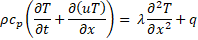
Assuming negligible viscous dissipation, the 1D instantaneous local energy balance equation for an incompressible pipe flow with constant fluid properties exhibits the following form:
where ![]() represents the bulk axial instantaneous air velocity, T the
bulk temperature of air,
represents the bulk axial instantaneous air velocity, T the
bulk temperature of air, ![]() the fluid density,
the fluid density, ![]() the specific heat at
constant pressure and
the specific heat at
constant pressure and ![]() the local specific convective heat transfer exchanged through the
perimeter of a pipe of length
the local specific convective heat transfer exchanged through the
perimeter of a pipe of length ![]() .
.
As proposed by Reynolds et al. [19], in the specific case of a turbulent pulsating flow, each of the flow properties can be decomposed into three different terms, as expressed in the following equation:

where ![]() represents the time-averaged
component only function of the x-axis,
represents the time-averaged
component only function of the x-axis, ![]() is the oscillating term
of the coherent cycle-stationary pattern and
is the oscillating term
of the coherent cycle-stationary pattern and ![]() corresponds to the
turbulent fluctuations term.
corresponds to the
turbulent fluctuations term.
Time
averaging ![]() determines
determines![]() and
the phase-average
and
the phase-average![]() , i.e. the average over a large ensemble of points having the same phase
with respect to a reference oscillator, leads to:
, i.e. the average over a large ensemble of points having the same phase
with respect to a reference oscillator, leads to:

Phase-averaging removes the background turbulence and extracts only the organized motions from the total instantaneous profile. For the sake of brevity, some useful mathematical properties that follow from the basic definitions of the time and phase averages are not reported here. They are detailed in [19].
Combining Eq.3 and Eq.2 and then applying the phase averaging operator to the equation obtained leads to:

In the left-hand side of
this equation, the sum of
the first two terms represents the rate of change of the air energy inside the
control volume (![]() is equal to zero because
of the time-independency of the component
is equal to zero because
of the time-independency of the component![]() ); the other terms
represent the advective transport of energy by mean flow, oscillating motion
and fluctuating motion through the control volume. In the right-hand side of the equation,
the sum of the first two terms corresponds to the conduction heat
flux through the control volume and the last term represents the phase-average of
the local convective heat transfer between the air and the solid wall. Time-averaging
Eq. 5 leads to:
); the other terms
represent the advective transport of energy by mean flow, oscillating motion
and fluctuating motion through the control volume. In the right-hand side of the equation,
the sum of the first two terms corresponds to the conduction heat
flux through the control volume and the last term represents the phase-average of
the local convective heat transfer between the air and the solid wall. Time-averaging
Eq. 5 leads to:
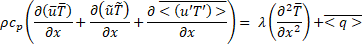
By integrating Eq. 6 on the volume defined by a cylinder of section ‘S’ and length ‘L’ (corresponding to the control volume, between the inlet and outlet measuring sections, in the following), the energy conservation equation can be written as:
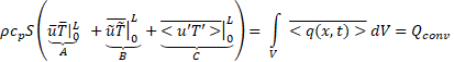
The total time-averaged convective heat
transfer ![]() is equal to the sum of
three different terms: the term ‘A’ which physically represents the energy
variation of the time-mean component of the flow across the pipe, the term ‘B’
which represents the energy variation due to the oscillating component of the flow
and the term ‘C’ corresponding to the advective transport of energy by
fluctuating motion due to turbulence fluctuations. The statement of Eq. 7
clarifies that, wheneer a direct measurement of
is equal to the sum of
three different terms: the term ‘A’ which physically represents the energy
variation of the time-mean component of the flow across the pipe, the term ‘B’
which represents the energy variation due to the oscillating component of the flow
and the term ‘C’ corresponding to the advective transport of energy by
fluctuating motion due to turbulence fluctuations. The statement of Eq. 7
clarifies that, wheneer a direct measurement of ![]() is not available,
instantaneous measurements of the air velocity and temperature are required to
correctly compute all the terms in the left-hand side of Eq. 7. In this study, as
previously presented, a water flow was used to cool the external surface of the
pipe. In addition to keeping the wall temperature cold, constant and quite
homogeneous in the pipe section where heat transfers are characterized, this
experimental setup allows
is not available,
instantaneous measurements of the air velocity and temperature are required to
correctly compute all the terms in the left-hand side of Eq. 7. In this study, as
previously presented, a water flow was used to cool the external surface of the
pipe. In addition to keeping the wall temperature cold, constant and quite
homogeneous in the pipe section where heat transfers are characterized, this
experimental setup allows ![]() to be evaluated directly from
the water temperature measurements. In this manner, it is possible to avoid performing
instantaneous measurements of the flow properties at the inlet and the outlet
of the test-section.
to be evaluated directly from
the water temperature measurements. In this manner, it is possible to avoid performing
instantaneous measurements of the flow properties at the inlet and the outlet
of the test-section.
5. Results and Discussion
5. 1. Acoustic Characterization of the Pipe
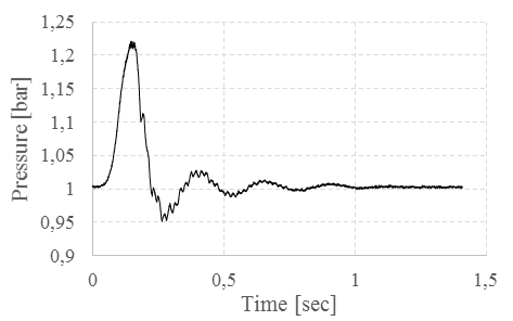
When the experimental apparatus is excited with an impulsive pressure source, the resonance frequencies of the system can be calculated by computing the power spectral density (PSD) of the pressure signal. These frequencies correspond to the local maxima of the PSD. In this study, a second order low-pass filter with a cut-off frequency of 1 kHz was applied to the sensor signals before calculating the PSD. Sensor signals were acquired at a frequency of 20 kHz, high enough to respect the Nyquist-Shannon sampling theorem. Because the behaviour of the pressure response to the impulsive pressure excitation is qualitatively the same for each pipe length, in the following figures only the pressure signal for one pipe length is shown. Figure 3 shows the instantaneous pressure, measured at the centre of the test-section, and figure 4 shows the PSD of the signal obtained for a specific pipe length. The other pressures, measured at different pipe axial positions or for the other pipe lengths, show the same PSD results and are not reported here. Local maxima of the PSD, identified by the red points on figure 4, correspond to the resonance frequencies of the system. Table 1 shows the first six calculated resonance frequencies for the three pipe lengths tested.
Results show that the first resonance mode
of the system is quite different from the resonance frequency calculated for a
pipe closed at one end and open to the surrounding air at the other end, which
is equal to ![]() , where
, where ![]() is a natural integer number equal to 1 for the first resonance
mode,
is a natural integer number equal to 1 for the first resonance
mode, ![]() is the sound speed and
is the sound speed and ![]() is the pipe length. This means that the volume of the outlet plenum
is not large enough to be representative of an open exhaust at pressure and
temperature ambient conditions. This implies that a
detailed numerical modeling of the experimental
apparatus should take into account this result through the
description of the boundary conditions.
is the pipe length. This means that the volume of the outlet plenum
is not large enough to be representative of an open exhaust at pressure and
temperature ambient conditions. This implies that a
detailed numerical modeling of the experimental
apparatus should take into account this result through the
description of the boundary conditions.
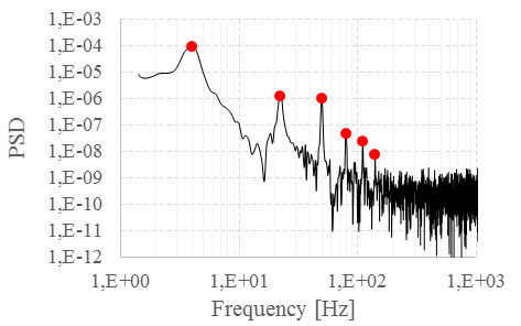
Table 1. Resonance frequencies [Hz] of the test-bench for different pipe lengths.
| Resonance Modes | 1 | 2 | 3 | 4 | 5 | 6 |
| L = 3.69m | 6.4 | 36.1 | 79.6 | 126.3 | 176.2 | 239.8 |
| L = 4.69m | 4.7 | 26.2 | 63.1 | 101.3 | 138.9 | 175.8 |
| L = 5.91m | 3.9 | 22.2 | 49.5 | 80.5 | 110 | 139.8 |
5. 2. Pulsation Effects on Convective Heat Transfers
As previously mentioned, given the
difficulty of measuring the three terms in the left-hand side of Eq. 7 experimentally,
the total time-averaged convective heat transfer ![]() was evaluated from the
water temperature measurements. In practice, a constant water volumetric flow
rate of 4.74 dm3/min is forced to pass through an annular section,
with an internal diameter of 67.3 mm and a thickness of 7 mm, in order to cool
the pipe wall. In these operating conditions, the Reynolds number of the water
flow is 788, leading to a laminar velocity profile under steady state
conditions. Consequently, from the energy balance equation for the water, in
which the convective heat transfer with the exterior ambient air was estimated
to be less than 10 W and was therefore neglected,
was evaluated from the
water temperature measurements. In practice, a constant water volumetric flow
rate of 4.74 dm3/min is forced to pass through an annular section,
with an internal diameter of 67.3 mm and a thickness of 7 mm, in order to cool
the pipe wall. In these operating conditions, the Reynolds number of the water
flow is 788, leading to a laminar velocity profile under steady state
conditions. Consequently, from the energy balance equation for the water, in
which the convective heat transfer with the exterior ambient air was estimated
to be less than 10 W and was therefore neglected, ![]() can be solved as the
time-averaged enthalpy difference of the water between the inlet and the outlet
of the test-section.
can be solved as the
time-averaged enthalpy difference of the water between the inlet and the outlet
of the test-section.
The air steady turbulent state (for the
particular case with a time-averaged Reynolds number of 30000) is taken as the
reference case. In such particular conditions, the term ‘B’ in Eq. 7 is null,
making it possible to compare ![]() computed from experiments
to the theoretical predicted one. The Nusselt number was evaluated using the
Colburn and the Dittus-Boelter correlations and applying the Bhatti and Shah
corrective coefficient [20] to take entry effects into account. For
a Re of 30000, the space-averaged Nusselt number was found to be equal to 89.4
with the Colburn correlation and 92 with the Dittus-Boelter correlation. The
total convective heat transfer linked to the Colburn correlation is 482 W,
which corresponds to a difference of 2.7% with the experimental value. With the
Nusselt number calculated from the Dittus-Boelter correlation the agreement is
even better, with a difference of less than 1%. Consequently, the small
differences between the theoretical predictions and the experiment validate the
evaluation of the total convective heat transfer based on water temperature
measurements.
computed from experiments
to the theoretical predicted one. The Nusselt number was evaluated using the
Colburn and the Dittus-Boelter correlations and applying the Bhatti and Shah
corrective coefficient [20] to take entry effects into account. For
a Re of 30000, the space-averaged Nusselt number was found to be equal to 89.4
with the Colburn correlation and 92 with the Dittus-Boelter correlation. The
total convective heat transfer linked to the Colburn correlation is 482 W,
which corresponds to a difference of 2.7% with the experimental value. With the
Nusselt number calculated from the Dittus-Boelter correlation the agreement is
even better, with a difference of less than 1%. Consequently, the small
differences between the theoretical predictions and the experiment validate the
evaluation of the total convective heat transfer based on water temperature
measurements.
A further comparison between ![]() and term ‘A’ in Eq. 7, in
the case of the steady turbulent flow, shows that the calculation of the
variation in the time-averaged enthalpy of air is not sufficient to correctly
compute the total time-averaged convective heat transfer: not taking into
account the turbulent term may lead to an underestimation of the total
time-averaged convective heat transfer of around 22%. The term ‘A’ was computed
by calculating the bulk flow temperature at the test-section inlet and outlet.
and term ‘A’ in Eq. 7, in
the case of the steady turbulent flow, shows that the calculation of the
variation in the time-averaged enthalpy of air is not sufficient to correctly
compute the total time-averaged convective heat transfer: not taking into
account the turbulent term may lead to an underestimation of the total
time-averaged convective heat transfer of around 22%. The term ‘A’ was computed
by calculating the bulk flow temperature at the test-section inlet and outlet.
Figure 5 shows the term ![]() of Eq. 7 for different
time-averaged Reynolds numbers, evaluated at the pipe length of 5.91 m.
of Eq. 7 for different
time-averaged Reynolds numbers, evaluated at the pipe length of 5.91 m.
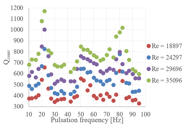
 for different time-averaged Reynolds numbers and pulsation frequencies.
 Results show that an increase in the time-averaged Reynolds number leads to an increase in the convective heat transfers, as could easily be deduced from a Nusselt correlation for a stationary turbulent flow. However, for particular excitation frequencies a strong heat transfer improvement occurs for all the tested mass flow rates, suggesting that the mechanism leading to this heat transfer enhancement is independent of the Reynolds number.
In order to understand this mechanism, the
time-averaged Nusselt number ![]() was
calculated in the particular case of a Re = 29696. It was evaluated by
modelling the heat transfer between the hot air and the water with three
thermal resistances placed in series to describe the internal forced convection
of the air, the radial conduction through the wall and the forced convection of
the water.
was
calculated in the particular case of a Re = 29696. It was evaluated by
modelling the heat transfer between the hot air and the water with three
thermal resistances placed in series to describe the internal forced convection
of the air, the radial conduction through the wall and the forced convection of
the water.
The air convective heat transfer
coefficient ![]() assumes
the following form:
assumes
the following form:

where ![]() and
and ![]() are the inner and outer
diameters of the annular section of the water, L is the length of the
test-section,
are the inner and outer
diameters of the annular section of the water, L is the length of the
test-section, ![]() is the thermal
conductivity of the wall,
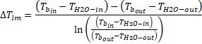
is the thermal
conductivity of the wall,![]() is the logarithmic
temperature difference usually used in the case of heat exchangers and
is the logarithmic
temperature difference usually used in the case of heat exchangers and ![]() is the convective heat
transfer coefficient of the
water. The latter was calculated according to the work of Dirker et al. [21], and
is the convective heat
transfer coefficient of the
water. The latter was calculated according to the work of Dirker et al. [21], and ![]() was calculated according
to the following equation:
was calculated according
to the following equation:
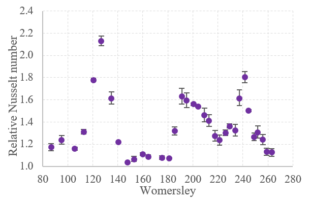
The relative time-averaged Nusselt number (defined
as the ratio of the time-averaged Nusselt number for the pulsating flow to the
corresponding one for a steady flow with the same time-averaged Reynolds number),
Nurel, is reported on figure 6 as a function
of the Womersley number for the experiment
corresponding to Re=29696 and for all the tested
frequency range. Uncertainties are depicted by error
bars in the figure. The Womersley number, defined as ![]() , which is a ratio of the
channel height to the Stokes boundary-layer thickness, is a dimensionless
expression of the pulsatile flow frequency in relation to viscous effects. L
represents the characteristic length of the system and for a pipe flow is equal
to the pipe internal diameter. The condition of no-slip at the wall
necessitates that for a pulsating flow, in order to accommodate the imposed
variation of flow rate additional vorticity must be generated in the boundary
layer in a manner which varies with time. Thus coherent shear waves are excited
which propagate from the wall into the fluid and are attenuated within a penetration
length. In the case of laminar pulsating flow, as
claimed from Uchida [22] the wave attenuation is characterized
by a length scale
, which is a ratio of the
channel height to the Stokes boundary-layer thickness, is a dimensionless
expression of the pulsatile flow frequency in relation to viscous effects. L
represents the characteristic length of the system and for a pipe flow is equal
to the pipe internal diameter. The condition of no-slip at the wall
necessitates that for a pulsating flow, in order to accommodate the imposed
variation of flow rate additional vorticity must be generated in the boundary
layer in a manner which varies with time. Thus coherent shear waves are excited
which propagate from the wall into the fluid and are attenuated within a penetration
length. In the case of laminar pulsating flow, as
claimed from Uchida [22] the wave attenuation is characterized
by a length scale ![]() (in which ν is the kinematic viscosity of the
fluid and ω is the angular
frequency of the pulsation). This length scale is usually referred to as the
Stokes layer thickness in recognition of the pioneering contribution which
Stokes made to the theory of unsteady flow.
(in which ν is the kinematic viscosity of the
fluid and ω is the angular
frequency of the pulsation). This length scale is usually referred to as the
Stokes layer thickness in recognition of the pioneering contribution which
Stokes made to the theory of unsteady flow.
Results show that for the entire Womersley range the relative time-averaged Nusselt number is always greater than 1: flow pulsation has a positive effect on heat transfers so that an enhancement of the internal forced convection, in comparison to the steady flow, is observed. This behaviour was found to be independent of the Reynolds number. According to the definitions of the Womersley number and of the Stokes layer, an increase of the pulsation frequency leads to a thinning of the viscous fluid boundary layer for the pulsating flow, which means that the velocity field is affected in a more restricted zone near the wall with the increase of Wo. However, in terms of heat transfer enhancement, local optimal values of the Womersley number exist for the maximization of the relative Nusselt number. This result indicates that the transport of energy and the transport of the momentum are differently impacted by the variation of the Womersley number. This result agrees with the experimental results in Ref. [11], where a local maximum in the heat transfer enhancement was found for a particular value of Wo. In the present study, these optimal values of Wo, where a local maximum of the relative time-averaged Nusselt number appears, correspond to pulsation frequencies identified as resonance frequencies of the system (that are 22.5, 50 and 80 Hz). Similar results were found by varying the pipe length for this time-averaged Reynolds number: for each of the pipe lengths tested when the flow is excited, with a pulsation frequency equal to one of the resonance modes, a heat transfer enhancement occurs. However, the magnitude of the heat transfer enhancement differs for each resonance mode and pipe length. This kind of result suggests that a coherent heat transfer enhancement mechanism exists when the flow is in resonant state.
To describe this mechanism, the instantaneous radial profile measurements of air velocity and temperature at the middle of the test-section (section B – B’ in Fig. 4) were analysed. Using the 1D assumption adopted, it is possible to calculate the local terms in the left side of Eq. 6. In order to be in agreement with the 1D approach, the physical quantities correspond to the integral of the measured profiles on the cross section.
Instantaneous measurements were conducted
only for pulsation frequencies below 30 Hz since the size of the thermocouple means
that measurements for higher frequencies cannot be exploited due to the time
constant of the thermocouple that cannot
be compensated using a Kalman filter method. The
measurement procedure of the instantaneous profiles of air axial velocity,
using hot-wire anemometry, and air temperature, with micro unsheathed
thermocouples, requires a correction of the hot-wire signals to account for the
temperature variation of air as well as a thermocouple signal compensation for
the sensor time delay. For frequencies higher than 30 Hz, the implicit
filtering of the real temperature variations, due to the thermal inertia of the
sensors, makes compensation of the thermocouple signal unfeasible, nor does it
allow temperature compensation of the hot-wire signal. The pulsation frequencies
below 30 Hz were chosen as a function of particular heat transfer conditions:
10 Hz and 12.5 Hz were selected for the light impact on heat transfers, 20 Hz
and 22.5 Hz because of their vicinity to the second resonance mode of the pipe,
and 30 Hz because it has the smallest relative Nusselt number. The term ![]() , which represents the
enthalpy transported by the time-averaged component of the flow, was found to
be slightly dependent on the pulsation frequency.
, which represents the
enthalpy transported by the time-averaged component of the flow, was found to
be slightly dependent on the pulsation frequency.
The term ![]() could not be computed
from the experimental results because of the impossibility of measuring the
turbulent components of the flow velocity and temperature. However, assuming that the variation in the pulsation frequency does not
significantly impact the turbulence properties, it can be considered that this
term will not modify the convective heat transfer when the pulsation frequency
is changed.
could not be computed
from the experimental results because of the impossibility of measuring the
turbulent components of the flow velocity and temperature. However, assuming that the variation in the pulsation frequency does not
significantly impact the turbulence properties, it can be considered that this
term will not modify the convective heat transfer when the pulsation frequency
is changed.
Since the Peclet number, defined as the ratio of the advection and diffusion rates of the thermal energy and equal to the product of the Nusselt and Prandtl numbers, is much higher than 1 in the present experimental conditions, heat transfers occur in a convective dominant regime and hence, the conduction term in Eq. 6 can be neglected.
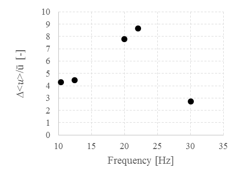
Finally, the results for the terms ![]() and
and ![]() are reported in the
following figures (Fig. 7 & Fig. 8).
are reported in the
following figures (Fig. 7 & Fig. 8). ![]() represents the weight of
the phase-averaged velocity oscillation amplitude on the time-averaged velocity
component and characterizes the increase in the oscillating component of the
flow due to pulsation.
represents the weight of
the phase-averaged velocity oscillation amplitude on the time-averaged velocity
component and characterizes the increase in the oscillating component of the
flow due to pulsation.
 as a function of the
pulsation frequency.
as a function of the
pulsation frequency.The results in figure 7 show a maximum of
the term ![]() corresponding to the
resonance frequency of the system, indicating that a flow resonance implies a
wide oscillating velocity component. Furthermore, since
corresponding to the
resonance frequency of the system, indicating that a flow resonance implies a
wide oscillating velocity component. Furthermore, since ![]() values are all higher
than 1, it can be concluded that flow reversal occurs for all the frequencies
analysed in figure 7, as confirmed by the instantaneous measurements of the air
velocity with the double wire probe.
values are all higher
than 1, it can be concluded that flow reversal occurs for all the frequencies
analysed in figure 7, as confirmed by the instantaneous measurements of the air
velocity with the double wire probe.
 as a function of
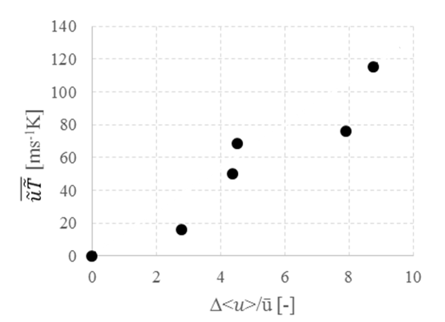
The results in figure 8 show the term ![]() as a function of
as a function of ![]() . By linking figures 7 and
8, it can be observed that large
velocity oscillations, which correspond to high
. By linking figures 7 and
8, it can be observed that large
velocity oscillations, which correspond to high ![]() values, are favoured for
pulsation frequencies close to the resonance frequency (the highest values of
values, are favoured for
pulsation frequencies close to the resonance frequency (the highest values of ![]() correspond to the
frequencies around the second resonance mode of the system, i.e. 22.5 Hz) and
lead to an increase of
correspond to the
frequencies around the second resonance mode of the system, i.e. 22.5 Hz) and
lead to an increase of ![]() as a function of
as a function of ![]() . The
linear trend that seems to emerge in figure 8 cannot be asserted because of the
frequency domain in which temperature and air velocity measurements have been
conducted is too narrow. The heat transfer enhancement
for these frequencies, observed on figure 6, is therefore mainly attributed to a
large oscillating component of the fluid velocity which increases the
oscillating heat advection.
. The
linear trend that seems to emerge in figure 8 cannot be asserted because of the
frequency domain in which temperature and air velocity measurements have been
conducted is too narrow. The heat transfer enhancement
for these frequencies, observed on figure 6, is therefore mainly attributed to a
large oscillating component of the fluid velocity which increases the
oscillating heat advection.
5. Conclusion
In this study, the heat transfer mechanism for a pulsating turbulent pipe flow has been investigated. A test-rig, designed to generate a pulsating hot air flow representative of the intake and exhaust of an internal combustion engine, has been presented, in which a pulsating turbulent hot air flow exchanges energy with a water cooled pipe with a pulsation frequency ranging from 10 to 95 Hz and a Reynolds number, based on the time-averaged velocity, ranging from 1.8 x10⁴ to 3.5 x10⁴. Three different pipe lengths were investigated.
Particular attention was paid to the calculation of the time-averaged convective heat transfer by developing an analytical formulation of the heat transfer problem for a 1D pulsating turbulent pipe flow. This development evidenced that whenever a direct measurement of the total time-averaged convective heat transfer is not available, instantaneous measurements of the air velocity and temperature are required to correctly compute the terms linked to the oscillating component of the flow in the energy balance equation.
Experimental results showed that the flow pulsation enhances heat transfers in the entire range of frequencies investigated for all the Reynolds numbers tested. Furthermore, for particular pulsation frequencies, the heat transfer improvement due to pulsation is higher than the heat transfer enhancement that can be achieved with a Reynolds number increase. In particular, it was experimentally observed that, when the flow is excited with a frequency equal to a resonance mode of the system, a strong increase in heat transfers occurs. Instantaneous measurements of air velocity and temperature demonstrated that the increase in the energy axial advection due to the oscillating component of the velocity is the major cause of the heat transfer enhancement. This behaviour was observed to be independent of the pipe length, and therefore independent of the acoustic resonance modes of the pipe. These results suggest that flow pulsation may be used as an active method for heat transfer enhancement.
In addition to the results presented in this paper, a radial transport enhancement of thermal energy during flow reversal was observed and will be studied and characterized with a 2D approach in future work.
Acknowledgements
This work was supported by the ‘OpenLab Energetics’ program, thanks to the partnership between the Groupe PSA and the PRISME Laboratory of the University of Orleans.
References
[1] S. D. Petkovic, R. B. Pesic, and J. K. Likic, “Heat Transfer in Exhaust System of a Cold Start Engine at Low Environmental Temperature,” Thermal Science, vol. 14, pp. 209-221, 2010.
[2] R. Host, P. Moilanen, M. Fried, and B. Bogi, “Exhaust System Thermal Management : A Process to Optimize Exhaust Enthalpy for Cold Start Emissions Reduction,” SAE Technical Paper, no. 2017-01-0141, 2017. View Article
[3] J. E. Dec, J. O. Keller, and V. S. Arpaci, “Heat transfer enhancement in the oscillating turbulent flow of a pulse combustor tail pipe,” International Journal of Heat and Mass Transfer, vol. 35, no. 9, pp. 2311-2325, 1992. View Article
[4] J. E. Dec and J. O. Keller, “Pulse combustor tailpipe heat-transfer dependence on frequency, amplitude, and mean flow rate,” Combustion and Flame, vol. 77, no. 3-4, pp. 359-374, 1989. View Article
[5] J. E. Dec, J. O. Keller, and I. Hongo, “TimeResolved Velocities and Turbulence in the Oscillating Flow of a Pulse Combustor Tail Pipe,” Combustion and Flame, vol. 83, no. 3-4, pp. 271- 292, 1991. View Article
[6] J. E. Dec and J. O. Keller, “Time-resolved Gas Temperatures in the Oscillating Turbulent Flow of a Pulse Combustor Tail Pipe,” Combustion and Flame, vol. 80, no. 3-4, pp. 358-370, 1990. View Article
[7] Y. Xu, M. Zhai, L. Guo, P. Dong, J. Chen, and Z. Wang, “Characteristics of the pulsating flow and heat transfer in an elbow tailpipe of a self-excited Helmholtz pulse combustor,” Applied Thermal Engineering, vol. 108, pp. 567-580, 2016. View Article
[8] M. Zhai, X. Wang, T. Ge, Y. Zhang, P. Dong, F. Wang, G. Liu, and Y. Huang, “Heat transfer in valveless Helmholtz pulse combustor straight and elbow tailpipes,” International Journal of Heat and Mass Transfer, vol. 91, pp. 1018-1025, 2015. View Article
[9] J. T. Patel and M. H. Attal, “An Experimental Investigation of Heat Transfer Characteristics of Pulsating Flow in Pipe,” International Journal of Current Engineering and Technology, vol. 6, no. 5, pp. 1515-1521, 2016.
[10] A. E. Zohir, “Heat Transfer Characteristics in a Heat Exchanger for Turbulent Pulsating Water Flow with Different Amplitudes,” Journal of American Science, vol. 8, no. 2, pp. 241-250, 2012.
[11] H. Li, Y. Zhong, X. Zhang, K. Deng, H. Lin, and L. Cai, “Experimental Study of Convective Heat Transfer in Pulsating Air Flow inside Circular Pipe,” in International Conference on Power Engineering, 2007, pp. 880-885. View Article
[12] M. A. Habib, A. M. Attya, A. I. Eid, and A. Z. Aly, “Convective heat transfer characteristics of laminar pulsating pipe air flow,” Heat and Mass Transfer, vol. 38, no. 3, pp. 221-232, 2002. View Article
[13] M. A. Habib, S. A. M. Said, A. A. Al-Farayedhi, S. A. Al-Dini, A. Asghar, and S. A. Gbadebo, “Heat transfer characteristics of pulsated turbulent pipe flow,” Heat and Mass Transfer, vol. 34, no. 5, pp. 413-421, 1999.
[14] T. Moschandreou and M. Zamir, “Heat transfer in a tube with pulsating flow and constant heat flux,” International Journal of Heat and Mass Transfer, vol. 40, no. 10, pp. 2461-2466, 1997. View Article
[15] S. A. M. Said, Al-Farayedhi A., M. Habib, S. A. Gbadebo, A. Asghar, and S. Al-Dini, “Experimental Investigation of Heat Transfer in Pulsating Turbulent Pipe Flow,” International Journal of Heat and Fluid Flow, p. 54, 2005.
[16] S. V. Nishandar and R. H. Yadav, “Experimental investigation of heat transfer characteristics of pulsating turbulent flow in a pipe,” International Research Journal of Engineering and Technology, vol. 2, no. 4, pp. 487-492, 2015.
[17] E. A. M. Elshafei, Safwat Mohamed, H. Mansour, and M. Sakr, “Numerical study of heat transfer in pulsating turbulent air flow,” Journal of Engineering and Technology Research, vol. 4, no. 5, pp. 89-97, 2012. View Article
[18] K. Kar, S. Roberts, R. Stone, M. Oldfield, and B. French, “Instantaneous exhaust temperature measurements using thermocouple compensation techniques,” SAE Technical Paper 2004-01-1418, pp. 169-190, 2004. View Article
[19] W. C. Reynolds and A. K. M. F. Hussain, “The mechanics of an organized wave in turbulent shear flow. Part 3. Theoretical models and comparisons with experiments,” Journal of Fluid Mechanics, vol. 54, no. 2, pp. 263-288, 1972. View Article
[20] John H. Lienhard, A heat transfer Textbook. p. 356, 2008.
[21] J. Dirker and J. P. Meyer, “Convective Heat Transfer Coefficients in Concentric Annuli,” Heat Transfer Engineering, vol. 26, no. 2, pp. 38-44, 2005. View Article
[22] S. Uchida, “The Pulsating Viscous Flow Superposed on the Steady Laminar Motion of Incompressible Fluid in a Circular Pipe,” Journal of Applied Mathematics and Physics, vol. 7, no. 5, pp. 403-422, 1956. View Article