Journal of Fluid Flow, Heat and Mass Transfer (JFFHMT)

ISSN: 2368-6111

Computational Fluid Dynamics of a Control Valve with Three-stage Perforated Cages under Varying Perforation Size Distributions

Yuki Kurosawa ¹, Chongho Youn¹

¹Azbil Corporation
1-12-2, Kawana, Fujisawa, Kanagawa, Japan 251-8522
y.kurosawa.a7@azbil.com; c.youn.9i@azbil.com

Abstract - The purpose of this study was to confirm, through experiments and computational fluid dynamics (CFD) analysis, the flow characteristics of a control valve with a three-stage perforated cage and to evaluate the flow state from the CFD visualization results. The control valve evaluated in this study was a size 2-inch perforated cage valve. We used a 3D metal printer to create two types of cages with different resistances in the first or second stage. The flow coefficient C_v was calculated from three differential pressure conditions, and the liquid pressure recovery factor F_L was calculated from the maximum differential pressure. We calculated and compared the flow characteristics, C_v and F_L, obtained from experiments and CFD analysis to confirm the validity of the CFD analysis model used in this study. We visualized the pressure distribution, velocity distribution, and void fraction obtained from the CFD analysis. The visualization results showed that the perforations in the first and second stages had non-choked turbulent flows with no cavitation, whereas perforations in the third stage had cavitation at the inlet of the perforations. We found that cavitation in the third stage could be suppressed by increasing the resistance of the first stage rather than increasing the resistance of the second stage. Specifically, increasing the resistance of the first stage reduced cavitation by 40% compared to increasing the resistance of the second stage.

Keywords: Control valve, Cavitation, CFD, Visualization

© Copyright 2025 Authors - This is an Open Access article published under the Creative Commons Attribution License terms Creative Commons Attribution License terms. Unrestricted use, distribution, and reproduction in any medium are permitted, provided the original work is properly cited.

Date Received: 2025-03-06
Date Revised: 2025-09-10
Date Accepted: 2025-09-27
Date Published: 2025-10-14

1. Introduction

Control valves are fluid machines used to control the flow rate and pressure of liquid flowing through pipes in chemical plants and factories. In particular, cavitation occurs in liquids owing to local increases in flow velocity and vortices, causing problems such as vibration and erosion. The intrinsic properties of a control valve include the flow coefficient C_V and liquid pressure recovery factor F_L. C_V indicates the ease of fluid flow, and F_L indicates the ease with which choke flow occurs owing to cavitation. Because control valves can also be used under high differential pressures, they must have a structure that suppresses cavitation. Therefore, research on cavitation suppression in control valves has been conducted. Previous research includes the following studies.

Gao et al. investigated cavitating flows in the orifices of poppet and ball valves using k–ε turbulence and multi-phase flow cavitation models [1]. Rammohan et al. investigated the effect of five types of cages with different numbers and types of perforations on flow rate and cavitation [2]. Maynes et al. investigated the flow through a perforated plate and found that the loss coefficient and cavitation number were highly dependent on the plate geometry [3]. Yaghoubi et al. studied the effects of the number of trims (no trim, one trim, and two and three trims) via numerical analysis [4]. Gao et al. experimentally and numerically investigated the flow and cavitation characteristics of cage-type control valves to identify the valve cages with better performance [5]. OU et al. performed three-dimensional simulations of cavitating flow in a pressure relief valve under different valve openings and visualized the flow to elucidate the cavitation distribution [6]. Sun et al. clarified the distributions of steam velocity, pressure, and turbulent kinetic energy in a multi-stage sleeve control valve at various opening degrees using numerical analysis [7].

In previous research, research has been conducted on the opening of multi-stage control valves or steam fluids. However, research on the effects of cavitation caused by the hole size distribution in multi-stage pressure reduction trims has not been found.

In this study, we used experiments and CFD to assess the influence of C_v and F_L on a three-stage perforated cage when the resistances of the first and second stages were changed. We compared the experimental flow characteristics and choke flow with the CFD analysis results to check the validity of the CFD analysis. We then visualized the pressure distribution, velocity distribution, and void fraction obtained from the CFD analysis to examine and assess the flow state inside the control valve and the location of cavitation occurrence.

2. Material and Method

2. 1. Control Valve

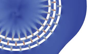
Fig. 1 shows a cross-sectional view of the 3D model of the perforated cage of the assessed 2-inch control valve, Fig. 2(A) shows an image of the perforated cage used in the experiment, Fig. 2(B) shows the details of the perforations in the perforated cage, and Fig. 2(C) shows a horizontal cross-sectional view of the perforated cage. The flow direction is indicated by an arrow in the figure and the valve is flow-to-close. In this study, we used two cages each with a three-stage structure created by a 3D metal printer. Because the cage perforations were created by a 3D metal printer, the top of the perforations had an acute angle, as shown in Fig. 2(A). The cage perforations were of two different sizes (Fig. 2(B)), and the area ratio of the large perforations to the small perforations was 1 : 0.7. The perforations were arranged in the first, second, and third stages from the outside of the cage toward the center, and the area ratios of each perforation for the two cage types are listed in Table 1. In the horizontal direction, the perforations were arranged every 12° in the first and third stages, whereas for the second stage, the perforations were arranged centrally between those in the first and third stages (Fig. 2(C)). In the vertical direction, each row comprised 3 perforations, and the perforation distance (distance between the centers of the semicircles) was 6.4 mm. Henceforth, the cage with small perforations in the first stage will be referred to as Model 1, and the cage with small perforations in the second stage will be referred to as Model 2. The valve travel in the experiment and CFD analysis was set to 100%.

Table 1. Perforation area ratio of perforated cages.

	1st stage	2nd stage	3rd stage
Model 1	0.7	1	1
Model 2	1	0.7	1

2. 2. Experimental Setup

Fig. 3 shows a schematic of the experimental equipment. Water was sent from the pump, and the flow rate was measured by a flow meter located on the inlet side of the test valve. The downstream valve was controlled to adjust the differential pressure applied to the test valve, and the flow rate, inlet pressure, differential pressure, and water temperature of the control valve were recorded after their values stabilized, and these values were used for the calculation of C_V and F_L. Water was sent to the water pool from the downstream valve and circulated. The pressure measurement points were set at 2D in the inlet side and 6D in the outlet side, where D is the pipe diameter, in accordance with the control valve test pressure measurement positions in International Electrotechnical Commission 60534-2-3.

C_V was determined from the non-choked flow state, and F_L was determined from the choked flow state. In this experiment, the inlet pressure P_in was set at 3.4 MPa (abs). C_V measurements were conducted under three differential pressure conditions, and F_L measurements were conducted at the maximum differential pressure achievable by the measurement equipment and at a differential pressure of 90% of the maximum differential pressure.

2. 3. CFD Analysis

In the CFD analysis, the pipe lengths on the inlet and outlet sides of the control valve were set to 2D and 6D, respectively, as in the experiment. Fig. 4 shows the CFD mesh. Fig. 5(A) shows the details of the perforations in the CFD mesh, and Fig. 5(B) shows an enlarged view of the perforations in the perforated cage. The upper acute angle of the perforations in the fabricated perforated cage was slightly flat; therefore, the perforations in the CFD mesh were filled in at 0.5 mm from the upper end. The mesh size was determined when generated to guarantee the greatest element resolution around the perforations. The 1D inlet pipe and 3D outlet pipe were created using a hexa mesh, and the other parts were created using a tetra mesh. The flow rate Q flowing into the control valve was calculated by applying the experimentally measured pressure conditions at the pipe inlet and outlet boundaries. CFD analysis was conducted by setting the intermediate differential pressure among the three differential pressure conditions as the boundary condition for C_V computations and the maximum differential pressure for F_L computations. C_V and F_L were determined by Eqs. (1) and (2) using each pressure P, flow rate Q, and saturated vapor pressure p_v.

(1)

(2)

Table 2 presents the details of the CFD analysis conditions. The CFD solver used was Advance/FrontFlow/Red Ver. 5.4, which is a commercial fluid analysis software developed by AdvanceSoft Corporation. This software supports parallel computation on supercomputers, enabling efficient large-scale simulations. A homogeneous flow model was used for cavitation modeling [8, 9]. The calculation was performed under the condition of incompressibility for C_V and compressibility for F_L. For the advection term, stable solutions were obtained using the second-order upwind method. In the CFD analysis of C_V,  was set at 1×10^-5, and in the CFD analysis of F_L, computations were conducted at 5×10^-6 to suppress computational divergence. Additionally, the number of mesh elements was set at approximately 7,000,000, and the computation was conducted using the supercomputer “Squid,” owned by Osaka University, which provided the computational resource. To ensure mesh independence, calculations were conducted with different mesh resolutions under identical conditions, and it was confirmed that the results did not depend on the mesh size.

Table 2. CFD conditions.

Software	Advance/FrontFlow/Red Ver.5.4
Turbulent model	Large Eddy Simulation (LES)
Fluid	Water (25℃) CV: Incompressible FL: Compressible
Number of cells	6,969,158 (Model 1) 7,115,330 (Model 2)
Advection term discrete scheme Momentum	2nd order upwind
Law of the wall	Spalding’s law
∆t	1×10-5, 5×10-6

3. Results and Discussion

3. 1. Experimental and CFD results

Fig. 6 shows the experimental and CFD analysis results for each cage. The vertical axis is the flow rate, and the horizontal axis is the 1/2 power of the differential pressure. The region where the flow rate increases linearly is a non-choked flow region, and the region where the flow rate remains unchanged is a choked flow region. No clear choked flow region, wherein the flow rate remains flat, was confirmed in either Model 1 or 2, which was consistent with the substantial experimental F_L results for Models 1 and 2.

Table 3 presents the experimental and CFD analysis results for C_V and F_L. The experimental F_L value for Model 1 exceeded the maximum measurable F_L (0.99) calculated from the upstream, differential, and saturated vapor pressures under the maximum differential pressure conditions achievable by the equipment. Therefore, the experimental F_L value for Model 1 was set at more than 0.99, and the CFD error was not calculated. The F_L for Model 1 was slightly higher than that for Model 2, indicating that the flow was less likely to choke. The errors between the experiment and CFD analysis were within 2.6% for C_V and 2.2% for F_L, and the CFS analysis model used in this study is thought to be valid.

Table 3. Results of the experiment and CFD analysis.

		CFD	Experiment	Error %
Model 1	CV	8.7	8.7	0.1
	FL	0.96	More than 0.99	-
Model 2	CV	8.7	8.9	-2.6
	FL	0.95	0.97	-2.2

3. 2. Visualization

Fig. 7(A) shows a vertical cross-sectional view of the center of the control valve, and Fig. 7(B) shows the top view of the horizontal cross-section on the straight red line indicated in Fig. 7(A). This horizontal cross-section was considered the second perforation cross-section from the top.

Fig. 8 shows the visualization results of the CFD analysis during F_L computation when the downstream pressure was set to atmospheric pressure to ensure the maximum differential pressure. Fig. 8 shows the results of the pressure, velocity, and void fraction of the area shown in Fig. 7(B). A comparison of the pressure values in Models 1 and 2 reveals that the pressure reduction patterns differed. Model 1 exhibited a large pressure reduction in the first stage, whereas Model 2 exhibited a large pressure reduction in the second stage. No major differences in the pressure distribution were observed after the second stage. A comparison of the velocities showed that Model 1 had a higher velocity in the first stage, whereas Model 2 had a higher velocity in the second stage. A comparison of the void fractions showed that the first and second stages in both Models 1 and 2 exhibited a non-choked turbulent flow state without the occurrence of cavitation, and the third stage had a high void fraction on the wall surface with the occurrence of cavitation.

Fig. 9 shows the visualization of the void fraction in the third stage in Models 1 and 2. Fig. 9 shows a visualization of the inside of the perforations every 90°, with the visualized areas numbered I to IV in a counterclockwise direction and circled in red. The range of the color bar in Fig. 9 is set to a range from 0 to 1 to analyze the amount of cavitation. Fig. 9 shows that Model 2 had a wider area with a high void fraction, with cavitation occurring at the inlet of the perforations.

Fig. 10 shows a quantitative comparison of the amount of cavitation in the third stage regions identified in Fig. 9. The void fraction images shown in Fig. 9 were converted into 8-bit grayscale images. Regions (I)–(IV) of the third stage in Fig.9 were extracted, and the integrated luminance values within each region were calculated using the image analysis software Fiji. Fig. 10 presents the ratio of integrated luminance values for Model 1 relative to Model 2 in each region, where a lower ratio indicates a smaller amount of cavitation in Model 1 compared to Model 2. The results reveal that, except for region (II), Model 1 generally exhibits a lower level of cavitation than Model 2, although there are differences among regions. In region (II), there is no significant difference in the amount of cavitation between Model 1 and Model 2. The average value obtained by dividing the total brightness of Model 1 by that of Model 2 was 0.6, indicating that cavitation was suppressed by approximately 40% in Model 1 compared to Model 2. Therefore, increasing the resistance of the first stage is thought to further suppress the occurrence of cavitation.

Fig. 11 shows the visualization results of the vertical cross-sectional view of the F_L CFD analysis. Fig. 11 shows that the height of the perforations had no effect on the pressure, velocity, or void fraction.

	Pressure
Model 1
Model 2
Color bar

	Velocity
Model 1
Model 2
Color bar

	Void fraction
Model 1
Model 2
Color bar

Figure 8. Horizontal cross-sectional view.

	I
Model 1
Model 2

 

	II
Model 1
Model 2

 

	III
Model 1
Model 2

	IV
Model 1
Model 2
Color bar

Figure 9. Visualization of the void fraction in the third stage.

	Pressure
Model 1
Model 2
Color bar

 

	Velocity
Model 1
Model 2
Color bar

	Void fraction
Model 1
Model 2
Color bar

Figure 11. Vertical cross-sectional view.

4. Conclusion

In this study, we used experiments and CFD analysis to assess the flow characteristics of a control valve when changing the resistance ratio of the first and second stages of the perforated cage having a three-stage structure. We obtained the following conclusions.

1. The F_L of Model 1, which had a larger resistance in the first stage, was higher than that of Model 2 and less likely to choke.
2. The visualization of Models 1 and 2 showed that the first and second stages exhibited non-choked turbulent flows in which no cavitation occurred.
3. We found that cavitation in the third stage could be suppressed by increasing the resistance of the first stage rather than increasing the resistance of the second stage. Specifically, Model 1 reduced cavitation by 40% compared to Model 2.

Acknowledgements

This work used computational resources of the Supercomputer Squid provided by Osaka University through the HPCI System Research Project. (Project ID: hp220116)

References

[1] H. Gao, W. Lin and T. Tsukiji, "Investigation of cavitation near the orifice of hydraulic valves Proceedings of the Institution of Mechanical Engineers," Part G: Journal of Aerospace Engineering, vol. 220, no. 4, pp. 253-265, 2006. View Article
[2] S. Rammohan, S. Saseendrans and S. Kumasaswamy. "Effect of multi jets on cavitation performance of globe valves," Journal of Fluid Science and Technology, vol. 4, no. 1, pp. 128-137, 2009. View Article
[3] D. Maynes, G. J. Holt and J. Blotter. "Cavitation inception and head loss due to liquid flow through perforated plates of varying thickness," Journal of Fluids Engineering, vol. 135, no. 3, 2013. View Article
[4] H. Yaghoubi, S. A. H. Madani and M. Alizadeh. "Numerical study on cavitation in a globe control valve with different numbers of anti-cavitation trims," Journal of Central South University, vol. 25, no. 11, pp. 2677-2687, 2018. View Article
[5] Z. Gao, Y. Yue, J. Wu, J. Li, H. Wu and Z Jin. "The flow and cavitation characteristics of cage-type control valves," Engineering Applications of Computational Fluid Mechanics, vol. 15, no. 1, pp. 951-963, 2021. View Article
[6] G. F. OU, J. Xu, W. Z. Li, B. Chen, "Investigation on Cavitation Flow in Pressure Relief Valve with High Pressure Differentials for Coal Liquefaction," Procedia Engineering, vol. 130, pp. 125-134, 2015. View Article
[7] Y. Sun, J. Wu, J. Xu, X. Bai, "Flow Characteristics Study of High-Parameter Multi-Stage Sleeve Control Valve," Processes, vol. 10, 1504, 2022. View Article
[8] Yuki Kurosawa, "Using Engineering Equation Solver (EES) to Solve Engineering Problems in Mechanical Engineering", Paper No. IMECE2018-86078, pp. V005T07A040; 4 pages, doi:10.1115/IMECE2018-86078, 2018 View Article
[8] Y. Saito, "Numerical analysis of unsteady vaporous cavitating flow around a hydrofoil," Fifth International Symposium on Cavitation (CAV2003), Osaka, Japan, 2003
[9] Y. Saito, R. Takami, I. Nakamori, T. Ikohagi, "Numerical analysis of unsteady behavior of cloud cavitation around a NACA0015 foil," Computational Mechanics, Vol. 40, pp. 85-96, 2007. View Article