Journal of Fluid Flow, Heat and Mass Transfer (JFFHMT)

ISSN: 2368-6111

1. Introduction

Issues such as the loss in the overall fuel cell performance, membrane and components degradation, and safety-related problems are some of the direct outcomes of the unintended diffusion of hydrogen gas from anode to the cathode. Thereby, they are collectively addressed through establishing a solid understanding about its mechanism and the extent of the implications of such phenomena to the overall fuel cell performance. Efficiency loss occur due to several factors. When hydrogen crossover (HCO) takes place, the diffused hydrogen does not participate in the primary electrochemical reaction desired for the generation of the overall electrical output; hence, a reduction in the available fuel for power generation. Also, heat is generated throughout the HCO process and cause several problems such as a decrease in the overall fuel cell efficiency as external systems are required to resolve the thermal management issues, the possibility of membrane and components deterioration due to localized heat accumulation, and the disruption of the operating conditions affecting the electrochemical reactions. Furthermore, mixed potential is one of the main consequences of HCO as “local cells” (or the segmented areas where HCO is measured) are observed to compete against the primary oxygen reduction reaction (ORR) [1]. On the other hand, fuel cell durability problems arise through chemical and mechanical pathways. Reactive oxygen species (ROS) and free radical formation happens which is responsible for the chemical degradation as they attack the polymer electrolyte membrane chains. Consequently, the catalyst materials are also targets to these attacks that, when prevalent, leads to a lower catalytic activity. Pinhole and crack formation are also associated with the HCO as the passage of hydrogen through the membrane introduce mechanical stress to its structure.

The direct implications of the HCO on the fuel cell performance are well-established; hence, the possibility of predicting the fuel cell performance as influenced by the temporal HCO is crucial in the study of its durability and lifetime estimation.  While it is noteworthy that predictive tools guide the development of more robust fuel cell systems, accurate and comprehensive modelling approaches must be prioritized for the simulation of long-term PEMFC performance and durability [2].

The effect of the HCO on OCV decay is not straightforward as it may seem. For example, Basha and Karan (2023) [3] found out that not all crossover hydrogen is fully oxidized in contrast to the general understanding that hydrogen reacts with the oxygen at the cathode side instantaneously; hence, necessitating the development of a more sophisticated model to account for the increased systemic complexity such as illustrated in their work [3]. Fully theoretical modelling approaches rely on various parameters and the development of a universally applicable model is mathematically challenging provided that all relevant phenomena must be considered to accurately predict the OCV decay against a set of predictors (e.g. HCO). Since these models are complex, oftentimes assumptions and simplifications are applied to rule out the majority of the model complexity. However, these may not hold true realistically in most cases as they are subject to researcher’s perspective which introduce some bias and could be responsible for the discrepancies between the predicted and the actual values. Ultimately, larger computational resources are pre-requisite to implement such simulation attempts [4].

Thus, data-driven approaches emerge in light of the challenges encountered with the theoretical modelling approaches. The growth of the studies exploring the direct application of machine learning (ML) models to PEMFC particularly on the durability and lifetime prediction has exponentially increased over the past decade. These models resolve the challenges of the trial-and-error experimentation as they allow rapid optimization and prediction tasks. In terms of dealing with multiple variables, ML models can capture complex, nonlinear behaviour in a particular dataset that the conventional fully theoretical models may struggle to carry out. Also, they are more adaptable to the introduction of new datasets and are scalable to handle big data. One skepticism towards ML models is that it may lack interpretability, and their results might not directly translate to the physical phenomena occurring inside the fuel cell. However, using algorithms to explain the ML models through measures such as Shapley values can help in determining how predictors influence the variability of the performance and durability of PEMFC. Since ML models act as surrogate models, they significantly reduce the cost when durability study is done experimentally and consequently reducing the development lead time. In terms of the accuracy, properly trained models with sufficient training data secures predictability with minimal errors. When usefulness is prioritized over interpretability, data-driven models can be practically suitable for carrying out optimization and prediction tasks. However, most ML models operate using large datasets to capture the latent features of the PEMFC operation but some models such as Gaussian Process Regression (GPR) generally performs well with small to moderate sized datasets as it incorporates operations on large covariance matrices. Depending on the type and volume of the dataset available, appropriate ML algorithms can be used to accurately predict the fuel cell performance, durability, and lifetime.

In this work, a GPR-based ML model was developed to predict the OCV decay as influenced by the temporal hydrogen crossover. To evaluate its performance, fit results, correlation coefficient, and statistical validation were carried out. The rationale of the predictive capability of the GPR-based model was established by correlating the model explanation results through Shapley values to the general knowledge about the relationship between temporal hydrogen crossover and OCV decay. Finally, the performance of the model during deployment was tested using a new dataset apart from the ones used during the model training and testing process. Essentially, this study is aligned with the results of Gomez et al. (2024) [5] wherein GPR-based model was found to generate the best predictive performance among the other ML-based models generated. The novelty in this work in comparison to their study lies in the interpretation of the model results against the physical understanding of the operations of a fuel cell system which was not carried out in the previous study. Overall, this work should provide not only a robust predictive tool for PEMFC but also the insights about the probable physical interpretation of the variances on the model prediction values.

2. Methodology

2.1. Data

The OCV decay against temporal hydrogen crossover data from Yao et al. (2024) [6] was used train, test, and validate the GPR model generated in this work.

Time and hydrogen crossover are the predictors, whereas OCV is the response variable in the dataset.

A total of 800 data points were generated wherein 480 were used to train the model, 160 were used for testing, and 160 were used for validation. Random sampling was employed in the selection of the data points for training, testing, and validation sets.

2. 2. Modelling Workflow, ML Algorithm, and Hyperparameters

2. 2. 1. GPR Algorithm

GPR algorithm was used to predict the OCV against time and hydrogen crossover current. GPR is a nonparametric, multivariate, probabilistic model based on Bayesian inference to predict not only the mean of the unseen data but also the uncertainty (variance) for each prediction [7]. This model follows a general linear regression model with Gaussian noise, given by (1):

(1)

(2)

where ε is the Gaussian noise, h(x)^T is the transposed vector form of the basis function, β is the vector of basis function coefficients, and f(x) is the zero-mean Gaussian Process with covariance (kernel) function k(x,x^') given by (2). ε follows a normal distribution as a function of mean and error variance, wherein mean is assumed to be zero. This relationship is given by (3):

(3)

where m(x) is the mean and σ² is the error variance. Overall, GPR is a probabilistic model where the response can be estimated using the conditional probability of y_i given f(x_i) and x_i for a normally distributed function provided by (4):

(4)

Equation (4) can be transformed to its vector form as shown in (5)-(6),

(5)

(6)

where covariance function is given by (7).

(7)

2. 2. 2. ML Framework

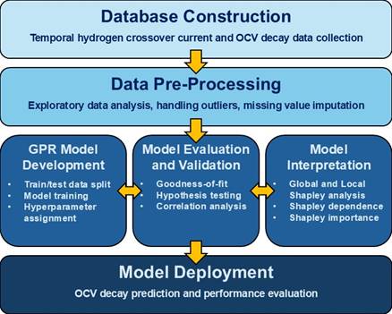
The ML modelling framework employed in this work is illustrated in Figure 1. Note that GPR model development, evaluation and validation, and interpretation is an iterative process, and the model could be improved through a continuous model fine-tuning.

2. 2. 3. GPR Hyperparameters

The hyperparameters used in developing the GPR model are summarized in Table 1 with their corresponding values and brief descriptions.

Table 1. GPR model hyperparameters.

Hyperparameter	Value	Description
Basis function	Constant	Assumes that the mean function is constant across all input points for model simplicity
Kernel function	Matérn 5/2	Kernel function under the Matern class with v (parameter that controls the smoothness of the resulting function) is 5/2
PredictMethod	Exact	Exact GPR method used when n ≤ 10,000
ActiveSetMethod	Random	Random active set selection
Beta	0.8958	Initial value of the basis function coefficient
Sigma	0.0010	Initial value of the Gaussian noise standard deviation
Loglikelihood	2792.1	Log marginal likelihood value used in the Bayesian hyperparameter optimization

The kernel function used in this work is the Matérn 5/2 covariance, a generalized form of Radial Basis Function (RBF) kernel with v=5/2 (twice differentiable functions) that is less smooth than RBF but more suitable in moderately smooth trends such as that observed in the dataset used in this work. The general form of the Matérn 5/2 covariance function is given by (8)

(8)

where σ_f is the signal standard deviation, σ_l the characteristic length scale, and r is the Euclidean distance between x_i and x_j as shown by (9).

(9)

2. 3. Model Performance Evaluation and Statistical Analysis

The objective of the GPR modelling is to minimize the loss function based on the mean squared error (MSE), given by (10), between the model and experimental OCV values as influenced by the temporal HCO. The root-mean-square error (RMSE) values for each observation were also determined as shown in (11). The goodness-of-fit and correlation are characterized by the coefficient of determination (R²) and correlation coefficient (R), respectively. The t-test results confirm if statistically significant difference exists between the model and experimental OCV values. Lastly, other statistical parameters such as the standard deviation and variance values were also calculated to inspect the spread of the data points for both the model and experimental datasets.

(10)

(11)

2. 4. Model Interpretation

The analysis of global and local Shapley values enables the understanding of the model prediction in relation to the physical phenomena occurring during the fuel cell degradation to address one main skepcticism about the application of any ML model to scientific projects: interpretability. Shapley values account for the effect of each predictor to the variability of the response variable for each prediction. Higher magnitude of Shapley values corresponds to greater influence of a predictor to the response. Similarly, the sign of a Shapley value tells if the variable positively or negatively influences the response. Around zero Shapley value, a predictor is observed to exhibit no influence on the variability of the response.

2. 5. Model Deployment

The performance of the developed GPR-based model was evaluated by using a new set of experimental data that was not used in training and testing processes. The metrics for the model performance during deployment were summarized.

3. Results and Discussions

3. 1. Model Performance

Table 2 summarizes the results of the GPR model’s fit performance, correlation, and statistical analysis. Based on the RMSE values, the model has performed exceptionally well across the training and testing. In fact, a slight improvement in the error was observed during model validation using the test dataset. R and R2 have values of 1.0000 and 1.0000, respectively, for both the training and test processes indicating a well-performing model.

Table 2. Performance and statistical analysis results.

Parameter	Training	Test
RMSE	6.2389E-05	5.6015E-05
R2	1.0000	1.0000
R	1.0000	1.0000
Null hypothesis	Not rejected	Not rejected
p-value	1.0000	0.1814
Standard deviation	0.04085	0.04032
Variance	0.0016688	0.0016257

 

Table 3. Model performance during deployment.

Parameter	Value
RMSE	6.78E-05
R2	1.0000
R	1.0000
Null hypothesis	Not rejected
p-value	0.3216
Standard deviation	0.039677
Variance	0.0015743

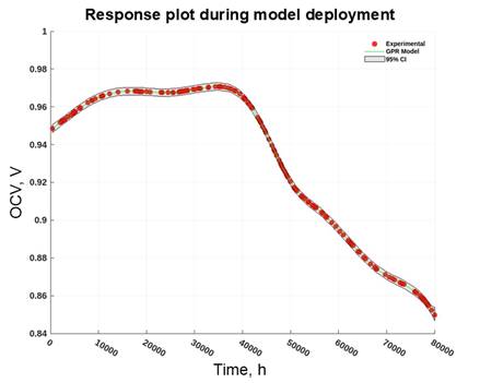
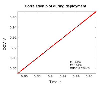
In terms of the statistical results, the null hypothesis was not rejected; meaning, there is no statistically significant difference observed between the model values and experimental data for both the training and test datasets. However, the p-value for the model prediction using the test dataset has seen to drop significantly, reducing the evidence to support the null hypothesis not being rejected. Nonetheless, the value still holds true for this criterion. In terms of the spread of the data, the variability of the model prediction during the training process is slightly higher than that of the test model prediction but this difference does not signify any huge effect on the model performance between the two processes. On the other hand, Table 3 shows the model performance during deployment. From these data, it is noticeable that a slight increase in the RMSE value can be observed. In terms of the p-value, a slight increase in the number was seen as well, strengthening the evidence to support the null hypothesis not being rejected. For the measures of spread, the values indicate smaller variability in the data. Figure 2 shows the response plot during the deployment giving the data for both the model and experimental values. Alongside, the uncertainty values for each observation were illustrated by the confidence interval as part of the output of a GPR-based model. From the trend of the data, it is evident that the model performed well in estimating the experimental data and that the uncertainty interval shows a narrow range which illustrates that the model predictions are of minimal uncertainty and that the probability that the model predictions to be the actual values of the unseen data is high. Although, the predictive capability of the model is valid only within the period of investigation (up to 80,000 hours) and may vary beyond that. The correlation plot in Figure 3 supports the excellent performance of the GPR model developed as experimental data lined up with the prefect prediction line. Therefore, there is strong evidence that the model could predict any intermediate value of the OCV within the period of analysis that were not captured during the experimental observations.

3. 2. Global and Local Interpretation of Model Predictions

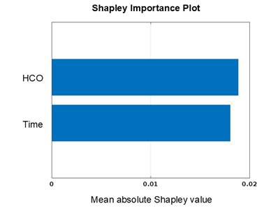
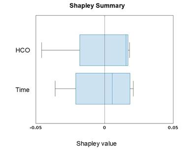
The extent to which a predictor influences the response variable is given by the Shapley Importance plot as shown in Figure 4. The plot illustrates that both HCO current and time almost equally influence the OCV based on the mean absolute Shapley values although a slightly greater importance was seen from the former. This indicates that both HCO and time explains the variability of the OCV values used in both the training and testing processes. In terms of the direction of their influence, Figure 5 illustrates the spread of the Shapley values for each predictor. It is apparent that HCO has a wider range of Shapley values than time although a narrower interquartile range (IQR) (between the 25th and 75th percentile) was seen which corresponds to a smaller variability in their values and that they are much more predictable and stable. Also, the distance between both the lower and upper bound of the IQR from the zero-value Shapley means that there is an equal likelihood that HCO influences the OCV positively and negatively based on the characteristics of the dataset. Interestingly, the blue vertical line within the box corresponds to the median Shapley values for each predictor. Given this, it is apparent that the Shapley values for HCO are, in many instances, has positive impact on the OCV which also means that across the entire dataset the model predicted HCO has generally improves them. This contrasts with what is known that HCO deteriorates the OCV. The explanation to this unusual observation is not yet known and would be challenging given the complexity of the PEMFC operation and that OCV is affected not only by the hydrogen crossover and time but many other factors all coming into play. Although, one thing that could explain this observed nuance is the distribution of the dataset to which the Shapley algorithm was tested. It is in fact that the trend of the OCV with HCO is not always increasing. Especially at the early stage of the accelerated stress test (AST) program [6], the OCV was found to be stable with HCO. Thus, it can be inferred that such trend seen could be due to how random sampling was done that the port-ion of the dataset wherein an increase in OCV with HCO was observed was therefore greater in number where the Shapley algorithm was tested. This observation was also observed from time as the influencing factor to OCV.

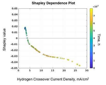
The Shapley Dependence plot, on the other hand, illustrates how Shapley values vary with both the HCO and time (shown in Figure 6). Based on this plot, it is observable that more Shapley values were under the zero-value Shapley, which indicates that most of the data suggesting the HCO and time to negatively influence the OCV which is aligned with the general understanding of how both parameters affects the PEFMC performance and durability [8]-[9]. The trend of the OCV data indicates how OCV decreases with increasing time and HCO values. In fact, the decrease in the OCV values were observed as early as 35,000 hours but a sharp decline in the values were seen between around 40,000 to 60,000 hours. Thus, it is evident that both time and HCO greatly influenced the OCV from these periods. On the other hand, the magnitude of the Shapley values within this period is at minimal. Thus, it can be interpreted that while the sharp decrease in the OCV values was observed during these hours of operations, there is weak evidence that both time and HCO could be the main cause of such decline and that the trend could be influenced and explained by other factors that were not considered in the dataset. To support this finding, Yao et al. (2024) [6] emphasized that aside from HCO, they also determined that the effect of decreasing shorting resistance at around 40,000 hours to the OCV was observed which could result to local overheating within the fuel cell and an increased hydrogen crossover flux due to membrane deterioration. As a recommendation, the authors pointed out that membrane shorting resistance should not go less than 1000 Ω-cm2. A similar study from Taylor et al. (2023) [10] has emphasized how changes in the membrane shorting resistance could greatly influence the OCV. In their work, it was noted that shorting resistance has created membrane failure points leading to premature OCV decline. Whereas, Lai and Fly (2015) [11] emphasized that there is no direct effect of shorting resistance to the OCV decay; rather, it highlighted that the implications of shorting resistance (e.g. membrane damage due to local heat generation) could eventually lead to the decline of the OCV. Other factors to consider include the integrity of the MEA setup, operating conditions, and the resistance of the fuel cell to chemical and mechanical degradation.

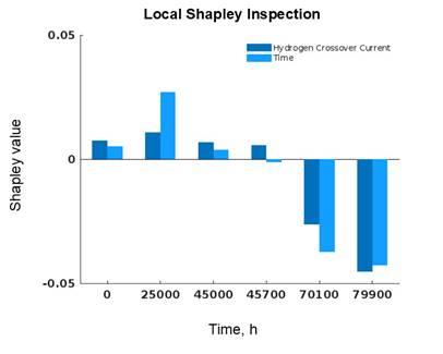
The local inspection of Shaley values across the dataset has provided useful insights into which predictor affects the variability of the OCV. Figure 7 shows the local Shapley values from different inspection points. At zeroth hour, the Shapley values for both the HCO and time are minimal and that HCO has a greater positive influence on the OCV. At 25,000 hours, the positive Shapley value for time is more than twice than that of the HCO. Notice that at around 45,700 hours, time starts to negatively impact the OCV while both predictors have a minimal effect to it. At 70,100 hours, both predictors were observed to significantly, negatively impacted the OCV values and that time dominated over the HCO. However, at the near end of the AST program, the HCO has greatly dominated the decline in the OCV values. It interesting to note that beyond the 40,000 hours of operation, the effect of both predictors on the OCV starts to manifest which is also aligned with what was observed experimentally. Overall, the local Shapley inspection not only provided the scale of the effects of both predictors to the OCV values, but it also aligns the capability of the model to predict the latent information about the relationship between these parameters which were not explicitly informed during the model training but was still captured by the model.

4. Conclusions

This work has successfully developed a GPR-based model to predict not only the OCV values as influenced by temporal HCO, but also the uncertainty measurements around each prediction. Furthermore, the model predictions were correlated with the Physics of the PEMFC performance degradation. Based on the fit performance, correlation analysis, and statistical validation, the model has consistently seen to perform well from training to deployment, with RMSE, R2, and R values of 6.78E-05, 1.0000, and 1.0000, respectively during the deployment, and that there is weak evidence to support the null hypothesis not being rejected given by the p-value of 0.3216. These measures were supported by how model predicted values have superimposed the perfect prediction line as the model was tested with new data. Furthermore, a narrow uncertainty interval was observed across all tested datapoints indicating that the model predictions could represent the values of the unseen OCV data. On the other hand, the Shapley values suggest that both HCO and time greatly influence the variability of the OCV values. In fact, it was noted that HCO has consistently dominated over time in terms of influencing the OCV values. Although, the Shapley summary indicates that both predictors have positive influence on the OCV in contracts to the general understanding that temporal HCO deteriorates the OCV and the reason behind is yet to be known. However, this was later contrasted by the observation on the Shapley dependence that most of these values were under the zero-line implying the negative impact of both parameters to the response variable. The local Shapley inspection uncovers that there is weak evidence that both predictors influence the OCV between 40,000 to 60,000 hours of operation by which was later confirmed that a significant decrease in the membrane shorting resistance could have predominated during these periods. At the near end of the AST program, both time and HCO exhibited great influence on the OCV decay wherein HCO predominated.

5. Future Direction

In terms of the general understanding of the PEMFC degradation, the OCV decay is collectively influenced by various factors and is not only limited to temporal HCO. Considering the consolidated influence of all possible degradation parameters could help the model understand and explain other latent features that were not covered in this work and would make it more robust in modelling the OCV decay. On the other hand, this work could be further extended by exploring how GPR model can predict values beyond the period of analysis used in the model training.

5. Acknowledgement

The authors acknowledge the Philippine Department of Science and Technology (DOST) for the financial support that this project under the Center for Advanced Materials and Clean Energy Technology (CAMCET) has received through the Niche Center for Research and Development in the Region (NICER).

References

[1] Tang, Q., Li, B., Yang, D., Ming, P., Zhang, C., & Wang, Y. (2021). Review of hydrogen crossover through the polymer electrolyte membrane. In International Journal of Hydrogen Energy (Vol. 46, Issue 42, pp. 22040-22061). Elsevier Ltd.
View Article
[2] Liu, D., & Case, S. (2006). Durability study of proton exchange membrane fuel cells under dynamic testing conditions with cyclic current profile. Journal of Power Sources, 162(1), 521-531.
[3] Basha, A. B. M., & Karan, K. (2023). Understanding Potential Decay during OCV Hold via Dry Recovery Process. Journal of The Electrochemical Society, 170(6), 064505. View Article
[4] Sugawara, S., Maruyama, T., Nagahara, Y., Kocha, S. S., Shinohra, K., Tsujita, K., Mitsushima, S., & Ota, K. ichiro. (2009). Performance decay of proton-exchange membrane fuel cells under open circuit conditions induced by membrane decomposition. Journal of Power Sources, 187(2), 324-331.
[5] Gomez, R. J., Apodaca, D., & Almendrala, M. (2024, August). Predictive Modelling of PEMFC Degradation Against Hydrogen Crossover Using Machine Learning Models in Matlab.
[6] Yao, Z., Zhou, F., Tu, C., Tan, J., & Pan, M. (2024). Decay behaviour of ultrathin reinforced membranes in PEMFCs subjected to the combination of mechanical/chemical accelerated stress testing. International Journal of Hydrogen Energy, 50, 200-208.
[7] Rasmussen, C. E., & Williams, C. K. I. (2006). Gaussian Processes for Machine Learning. The MIT Press.
[8] Rui, Z., Ding, R., Hua, K., Duan, X., Li, X., Wu, Y., Wang, X., Ouyang, C., Li, J., Li, T., & Liu, J. (2023). Design of proton exchange membranes with high durability for fuel cells: From the perspective of machine learning. Journal of Membrane Science, 683.
[9] Yoon, W., & Huang, X. (2010). Study of Polymer Electrolyte Membrane Degradation under OCV Hold Using Bilayer MEAs. Journal of The Electrochemical Society, 157(4), B599. https://doi.org/10.1149 View Article
[10] Taylor, A. K., Smith, C., & Neyerlin, K. C. (2023). Mitigation and diagnosis of pin-hole formation in polymer electrolyte membrane fuel cells. Journal of Power Sources, 571.
[11] Lai, Y. H., & Fly, G. W. (2015). In-situ diagnostics and degradation mapping of a mixed-mode accelerated stress test for proton exchange membranes. Journal of Power Sources, 274, 1162-1172.
[1] Tang, Q., Li, B., Yang, D., Ming, P., Zhang, C., & Wang, Y. (2021). Review of hydrogen crossover through the polymer electrolyte membrane. In International Journal of Hydrogen Energy (Vol. 46, Issue 42, pp. 22040-22061). Elsevier Ltd. View Article
[2] Liu, D., & Case, S. (2006). Durability study of proton exchange membrane fuel cells under dynamic testing conditions with cyclic current profile. Journal of Power Sources, 162(1), 521-531. View Article
[4] Sugawara, S., Maruyama, T., Nagahara, Y., Kocha, S. S., Shinohra, K., Tsujita, K., Mitsushima, S., & Ota, K. ichiro. (2009). Performance decay of proton-exchange membrane fuel cells under open circuit conditions induced by membrane decomposition. Journal of Power Sources, 187(2), 324-331. View Article
[5] Gomez, R. J., Apodaca, D., & Almendrala, M. (2024, August). Predictive Modelling of PEMFC Degradation Against Hydrogen Crossover Using Machine Learning Models in Matlab. View Article
[6] Yao, Z., Zhou, F., Tu, C., Tan, J., & Pan, M. (2024). Decay behaviour of ultrathin reinforced membranes in PEMFCs subjected to the combination of mechanical/chemical accelerated stress testing. International Journal of Hydrogen Energy, 50, 200-208. View Article
[7] Rasmussen, C. E., & Williams, C. K. I. (2006). Gaussian Processes for Machine Learning. The MIT Press. View Article
[8] Rui, Z., Ding, R., Hua, K., Duan, X., Li, X., Wu, Y., Wang, X., Ouyang, C., Li, J., Li, T., & Liu, J. (2023). Design of proton exchange membranes with high durability for fuel cells: From the perspective of machine learning. Journal of Membrane Science, 683. View Article
[10] Taylor, A. K., Smith, C., & Neyerlin, K. C. (2023). Mitigation and diagnosis of pin-hole formation in polymer electrolyte membrane fuel cells. Journal of Power Sources, 571. View Article
[11] Lai, Y. H., & Fly, G. W. (2015). In-situ diagnostics and degradation mapping of a mixed-mode accelerated stress test for proton exchange membranes. Journal of Power Sources, 274, 1162-1172. View Article