Journal of Fluid Flow, Heat and Mass Transfer (JFFHMT)
ISSN: 2368-6111

Volume 11 - Year 2024 - Pages 376-387
DOI: 10.11159/jffhmt.2024.037
Power Enhancement and Energy Efficiency of a Wind Turbine Equipped with a Slotted Jet: 3D-DDES Numerical Simulations of the S809 Airfoil
Giacomo Tosatti1, Luca Manni1, Ivano Petracci1*
1Department of Industrial Engineering, University of Rome “Tor Vergata”,
via del Politecnico n.1, 00133 Rome, Italy
*Corresponding author: ivano.petracci@uniroma2.it
giacomo.tosatti@students.uniroma2.eu
luca.manni@uniroma2.it
Abstract - Renewable energy sources are increasingly meeting global energy demands, with solar power leading the way and being closely followed by wind energy. For this reason, scientific research is focused on finding new ways to maximise the power generated by wind turbines, utilising both passive and active circulation control devices. This paper aims to investigate the aerodynamic performance of the NREL Phase VI wind turbine using the blade element momentum (BEM) theory and computational fluid dynamics (CFD). The baseline configuration, consisting of an S809 airfoil, is modified to employ trailing edge blowing technology, an active circulation control technique known as Coanda Jet. Calculations are performed via 3D Delayed Detached Eddy Simulation (DDES) to solve the three-dimensional flow structures over the airfoil correctly. Variations in chord and twist angle along the blade’s radius are taken into account by analysing five distinct radial positions and, by using Blade Element Momentum (BEM) theory, the total power output generated by the wind turbine is calculated. Simulations are performed at a fixed absolute wind speed equal to 7 m/s, both with and without jet blowing, employing three different jet momentum coefficients Cµ to evaluate the improvements in the examined sections' aerodynamic performance and assess the energy efficiency of the used technology. Results indicate a notable increase in lift, which consequently enhances both torque and thrust, leading to a net power gain of up to 25.1% compared to the baseline case.
Keywords: Wind Turbine; S809 Airfoil; Circulation Control; Jet Blowing; 3D-DDES simulation; Power Enhancement
© Copyright 2024 Authors - This is an Open Access article published under the Creative Commons Attribution License terms. Unrestricted use, distribution, and reproduction in any medium are permitted, provided the original work is properly cited.
Date Received: 2024-01-12
Date Revised: 2024-09-24
Date Accepted: 2024-10-04
Date Published: 2024-10-18
1. Introduction
Fossil fuels have always been humanity’s main source of energy power. However, researchers focused on new sources such as renewables due to their finite nature and the increasing necessity of lowering CO2 emissions coupled with a growing demand for energy production. Among all the environmentally friendly alternatives, wind energy stands as the second most prominent, preceded only by solar power [1]. As of June 2023, global installed wind power capacity reached 976 GW, and by the end of the year, an additional growth to 1045 GW is expected, with China and the USA composing more than 50% of it, followed by a large number of European countries [2]. Given the extensive use of wind turbines and the consequent investment in the order of billions of dollars [3], it is only evident why intensive efforts have been undertaken to maximise energy conversion efficiency, an objective satisfied by the employment of the so-called passive and active flow control devices, whose purpose is increasing the lift force which is in turn strictly related to power. The former consists of a simple modification of the airfoil geometry (flaps, slats, vortex generators), while the latter implies the expense of power provided by an external source, such as a compressor, to further increase the generated one: it is the case of jet blowing, or Coanda jet. This technology was born in aeronautics [4] and has been widely studied, as far as jet thickness, momentum and trailing edge radius are concerned by Djojodihardjo et al. [5] for wind turbine applications. It consists of the injection of pressurized fluid along the suction side, usually in close proximity to the airfoil’s trailing edge, with the goal of re-energizing the boundary layer to resist typical adverse pressure gradients delaying stall [6],[7] and, most importantly, forcing the surrounding fluid to adhere to the curved surface, increasing the circulation of velocity and thus lift force, as explained by the Kutta-Žukovskij’s theorem [8]. However, it must be noted that implementing trailing edge blowing implies its rounding, leading to an amplification of drag force, a problem that can be mitigated by designing its lower part as flat as possible, as suggested by Englar in [9]. Since airfoil geometry also plays a fundamental role, researchers have conducted numerous studies on its optimisation to pursue a compromise between lift and drag generation. An example is the S809 airfoil, designed by Somers in 1997 explicitly for wind energy application and tested in the low-turbulence wind tunnel of the Delft University of Technology Low-Speed Laboratory [10]. The specified airfoil was subsequently integrated into the NREL Phase-VI wind turbine, devised explicitly for experimental investigations, and tested by Hand et al. [11] in the NASA Ames Research Center’s wind tunnel, characterised by a 24.4 m x 36.6 m test section and a maximum wind speed of 50 m/s.
This work aims to further expand on the results obtained by Petracci et al. [12] and Tosatti et al. [13], by studying a three-dimensional flow and a broader range of jet velocities to demonstrate the attractiveness of the blowing technology. First, a series of preliminary 3D simulations are carried out, for a fixed absolute wind speed V = 7 m/s, on the airfoil at the r/R = 0.75 position of the blade’s radius without the jet, aiming to demonstrate mesh reliability and results are confronted with those of Somers for validation. The investigation is then extended to the five radial positions along the blade for which experimental data is available [11] and, through the use of Blade Element Momentum theory (BEM), generated power is evaluated in both jet-off and jet-on configurations to highlight its increase and prove the energy efficiency of the lift-increasing method.
2. Numerical methodology
2.1 Governing equations
The core equations descriptive of the problem are the first and second Navier-Stokes equations, nominally conservation of mass and momentum. Assuming the fluid to be incompressible, they can be written in their instantaneous form respectively as:

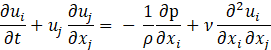
where xi represents the i-th coordinate, ui the i-th instantaneous velocity component written in a Cartesian reference frame, p is the instantaneous static pressure, ρ the density of the fluid and ν the kinematic viscosity. It is well known that the flow regime transitions from laminar to turbulent after a certain value of the Reynolds number, defined in Eq. 3:

where L is a characteristic dimension of the problem. This transition implies random changes in the instantaneous flow variables and, according to the turbulence description given by Kolmogorov in [14], it is only evident why a direct approach to solve the equations mentioned above via Direct Numerical Simulation (DNS) is deemed impractical, primarily due to the substantial time and computational resources required. A well-established method consists in performing the Reynolds average and so obtaining the Unsteady Reynolds-Average Navier-Stokes equations (URANS):

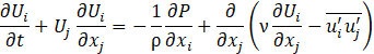
where Ui and Pi are the mean values of velocity and pression and the term ![]() consists in the apparent Reynolds stresses, caused by the fluctuations of velocity in the mean flow. This term adds new unknown variables, hence the need to model it by introducing new equations. Another technique is the Large Eddy Simulation (LES), which consists of a direct numerical solution of the large eddies and modelling smaller ones with Sub-Grid Scale models. They are easier to predict thanks to their almost-isotropic nature. This filtering operation is done through a spatial filter (i.e. mesh resolution) [14]. It is noteworthy that, while not as demanding in terms of time and resources as DNS, this approach is still relatively costly, so its use is mainly limited to academic research. This problem arises from the filtering operation itself, since wall-parallel grid dimensions become as crucial as wall-normal ones; a problem URANS does not encounter. In the present work a DES approach is chosen. Developed by Spalart in 1997 [15] and known as DES97, it consists in a hybrid RANS-LES approach: URANS is applied in the boundary layer where an onerous grid resolution would be required to solve the smaller scales born through the wall-flow interactions, modelling them instead; LES is used away from the wall. This method is, however, highly grid-dependent: a mesh fine enough to enter the boundary layer but not fine enough for accurate computation of the Reynolds stresses can cause the so-called Modelled Stress Depletion [17], resulting in an artificial flow detachment [18]. The Delayed Detached Eddy Simulation was so proposed by Spalart et al. in [19] to avoid this issue, a result obtained by modifying the definition of the length scale as shown below. In this work the k−ω SST turbulence model proposed by Menter [20] is employed to model the boundary layer. The transport equations of the turbulent kinetic energy k and the rate of dissipation ω necessary to model the term
consists in the apparent Reynolds stresses, caused by the fluctuations of velocity in the mean flow. This term adds new unknown variables, hence the need to model it by introducing new equations. Another technique is the Large Eddy Simulation (LES), which consists of a direct numerical solution of the large eddies and modelling smaller ones with Sub-Grid Scale models. They are easier to predict thanks to their almost-isotropic nature. This filtering operation is done through a spatial filter (i.e. mesh resolution) [14]. It is noteworthy that, while not as demanding in terms of time and resources as DNS, this approach is still relatively costly, so its use is mainly limited to academic research. This problem arises from the filtering operation itself, since wall-parallel grid dimensions become as crucial as wall-normal ones; a problem URANS does not encounter. In the present work a DES approach is chosen. Developed by Spalart in 1997 [15] and known as DES97, it consists in a hybrid RANS-LES approach: URANS is applied in the boundary layer where an onerous grid resolution would be required to solve the smaller scales born through the wall-flow interactions, modelling them instead; LES is used away from the wall. This method is, however, highly grid-dependent: a mesh fine enough to enter the boundary layer but not fine enough for accurate computation of the Reynolds stresses can cause the so-called Modelled Stress Depletion [17], resulting in an artificial flow detachment [18]. The Delayed Detached Eddy Simulation was so proposed by Spalart et al. in [19] to avoid this issue, a result obtained by modifying the definition of the length scale as shown below. In this work the k−ω SST turbulence model proposed by Menter [20] is employed to model the boundary layer. The transport equations of the turbulent kinetic energy k and the rate of dissipation ω necessary to model the term ![]() in the URANS part are respectively:
in the URANS part are respectively:
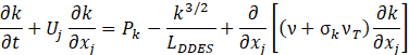

where LDDES is the integral length scale, dependent on the turbulent length scale of the k − ω SST Lt and the maximum grid dimension Δmax, defined in Eq. 8; νT is the turbulent kinematic viscosity and Pk is the production limiter, whose purpose is to avoid excessive build-up of turbulent kinetic energy near stagnation points at the leading edge of an airfoil:where LDDES is the integral length scale, dependent on the turbulent length scale of the k − ω SST Lt and the maximum grid dimension Δmax, defined in Eq. 8; νT is the turbulent kinematic viscosity and Pk is the production limiter, whose purpose is to avoid excessive build-up of turbulent kinetic energy near stagnation points at the leading edge of an airfoil:

with this length scale definition, when fd is 1 the model behaves as a LES and transitions to a RANS model when fd is 0. More insights about the variables and constants in Eq. 6, 7, 8 can be found in [21].
2.2 Grid generation
The original S809 airfoil with a chord length of 0.482 m has been modified to integrate the Coanda technology. The jet exit is placed at 95% of the chord c and its thickness tj is selected to obtain a ratio tj /c = 0.2%. The trailing edge was subsequently shaped by rounding and truncating to create a semi-circumference so that tj/RTE = 0.2, where RTE is the trailing edge’s radius, leaving the pressure side’s part flat as recommended by Englar in [4]. An O-mesh block strategy has been chosen to minimize element skewness and ensure orthogonality near the blunt edges of the trailing edge. It consists of a radius R = 50 c circumference centred on the airfoil’s leading edge to guarantee the independence of the turbulent quantities concerning the inlet boundary condition. Similarly, this extension also ensures a correct development of the wake, avoiding contaminations arising from the pressure imposed on the outlet boundary condition. Then, an auxiliary O-grid with a radius of r = 4 c is created to obtain a finer mesh near the airfoil and a controlled growth ratio. The mesh is then extruded in the spanwise direction for a length of 0.5 c. A velocity v = 29.3 m/s is imposed on the inlet, and a gauge pressure p = 0 Pa is on the outlet. The velocity mentioned above guarantees a Reynolds number evaluated with the chord Re ≈ 0.9·106, hence the choice to use Somers’ results as a benchmark for validation given that his Reynolds number, equal to Re = 1·106, is the closest available in the literature to the one adopted in this work. A translational periodic boundary condition is imposed on the front and back faces of the domain to emulate an "infinite" blade, as described by Eq 9:
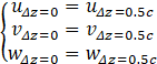
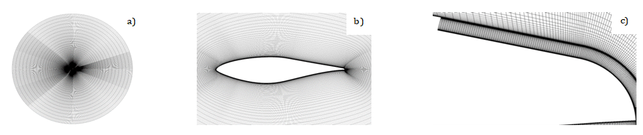
where u, v and w are the streamwise, wall-normal and spanwise velocities on the two lateral faces of the domain Δz= 0 and Δz= 0.5 c. The height of the first cell near the profile is fixed to achieve a y+ < 1 and the growth ratio is chosen to be ≤ 1.15. It should be noted that two extra blocks are needed to mesh the trailing edge and, given its particular geometry, it was necessary to transform the last square block into a triangular one. The grid resolution study has been carried out for an angle of attack α=14° for three different meshes, whose details are reported in Table 1, while the employed mesh of the domain and a closeup of the airfoil can be seen in Figure 1a and Figure 1b respectively. The results of the three simulations are reported in Table 2. The medium-resolution mesh was selected for the remaining simulations due to the close resemblance of the lift coefficients CL between the medium and the fine resolution. The jet canal, shown in Figure 1c, is later modelled on the pre-existing mesh by adding a new block whose length is ten times the thickness. It is then segmented with 70x70x64 points in the streamwise, normal, and spanwise directions, respectively. A no-slip boundary condition, described by Eq. 10, is applied both to the jet canal and the airfoil:

where τwall is the wall shear stress. The time step adopted is ∆t = 1·10−4 s to guarantee a CFL<1 at least in the LES region, while keeping it < 5 in the RANS region. As far as spatial discretisation is concerned, turbulent kinetic energy and specific dissipation rate are treated with a Second Order Upwind scheme, while momentum is treated with a Bounded Central Differencing scheme. The flow is assumed incompressible, hence the decision to treat pressure-velocity coupling with the SIMPLE algorithm [22]. Lastly, time is discretised via a Bounded Second Order Implicit scheme. Every simulation carried out in Ansys FLUENT, is run for 1.6s to eliminate any influence of the initialisation conditions, following which average quantities are monitored for an additional 3.2s, corresponding to two domain laps.
Table 1: Details of the three meshes for the baseline S809 airfoil
|
Parameters |
Coarse |
Medium |
Fine |
|
Normal points in R |
40 |
50 |
60 |
|
Normal points in r |
100 |
120 |
140 |
|
Growth ratio in R |
1.1 |
1.1 |
1.1 |
|
Growth ratio in r |
1.15 |
1.1 |
1.05 |
|
Wrap-around points |
340 |
520 |
660 |
|
Spanwise points |
64 |
64 |
64 |
|
y+ |
< 1 |
< 1 |
< 1 |
Table 2: Comparison of the aerodynamic coefficients
|
Results |
Coarse |
Medium |
Fine |
Exp. [10] |
|
CL |
0.957 |
0.998 |
1.012 |
1.055 |
|
CD |
0.0932 |
0.0793 |
0.0764 |
0.0828 |
2.3 Mesh validation
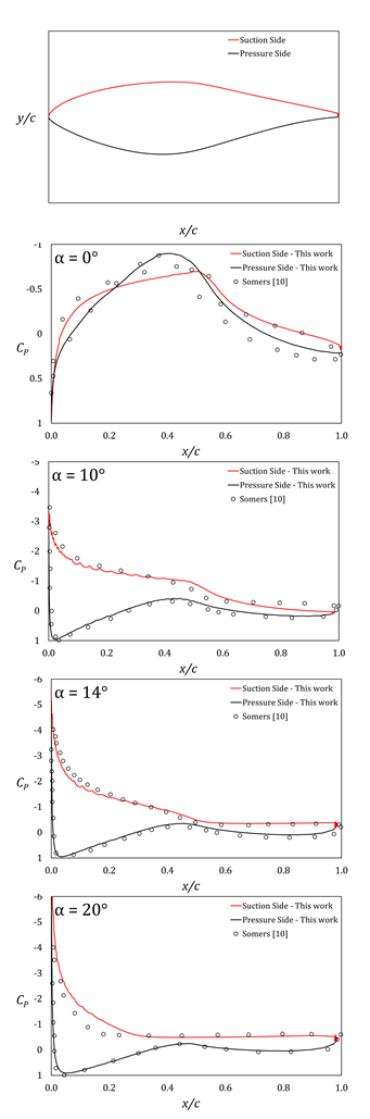
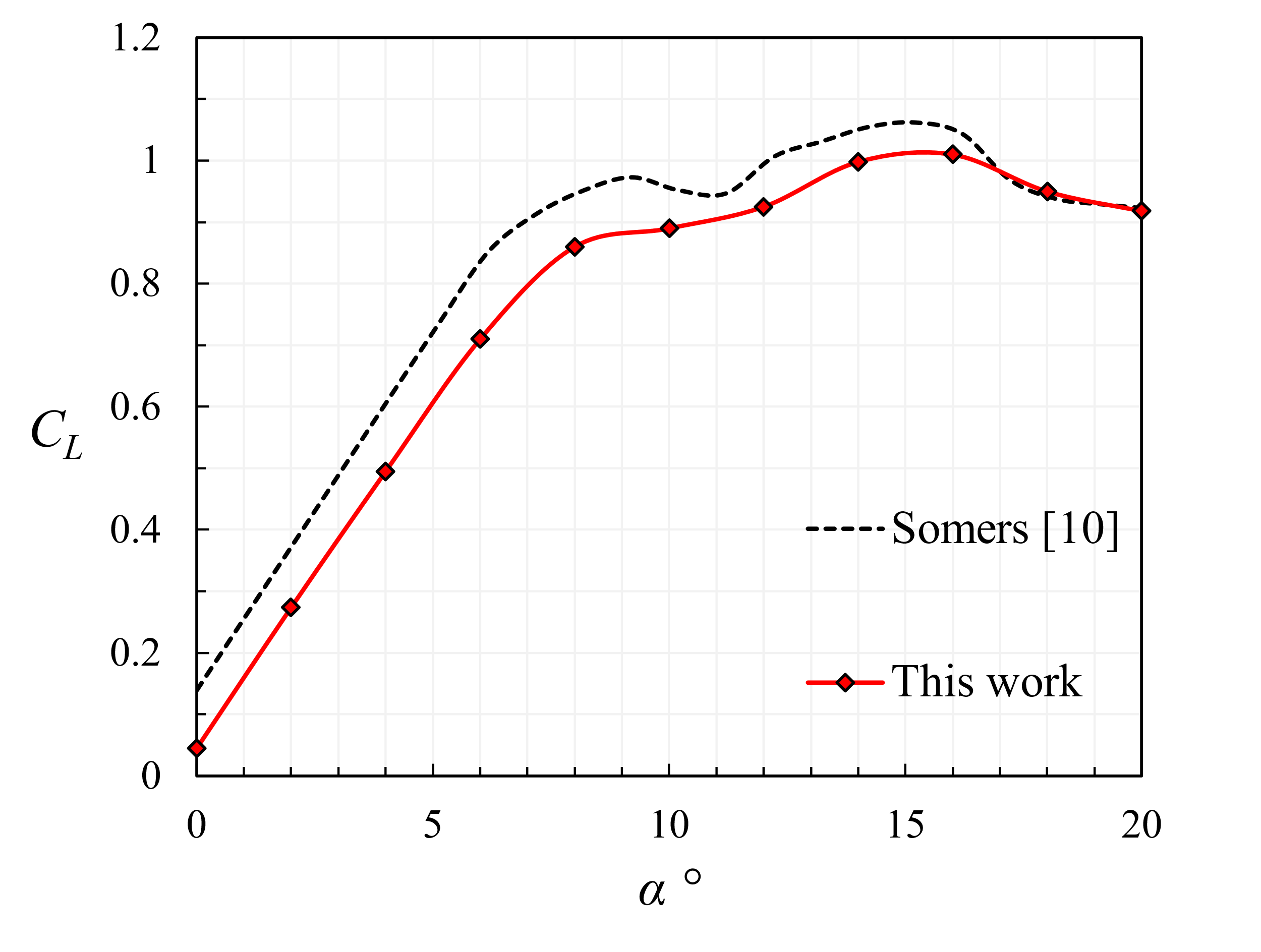
Figure 2 compares pressure coefficients with Somers' for four tested angles, agreeing well with the experimental results. Moreover, a wide range of angles of attack has been tested, spanning from 0° to 20° in increments of two. As shown in Figure 3, the lift curve closely follows Somers’ in shape; the discrepancy is found in the intensity of CL. The author believes this is caused by the difference in Reynolds number between the simulations presented in this work and, most importantly, by the effect of wall interference typical of subsonic wind tunnels [23]. However, given the nearly identical slope in the linear part of the curve from α = 0° to α = 6°, the similarity in the first-stall region from α = 8° to α = 12° as well as the subsequent recovery and deep-stall, results were deemed satisfactory.
2.4 Blade Element Momentum Theory
In the Blade Element Momentum theory, momentum and the blade’s rotation are considered, and the rotor is simplified to a series of independent annular rings. It should be noted that this theory overpredicts power generation because it does not account for wake expansion, tip losses, radial pressure gradients and blade interaction. However, it is still a powerful tool. Figure 4 clearly shows the correlation between the lift L and drag D coefficients, defined in Eq. 11 and Eq. 12, with the torque Tq and thrust Th, hence the definition of the torque and thrust coefficients CTq and CTh in Eq. 13 and Eq. 14.


Where θ is the sum of pitch and yaw angle and Aref is the planform area, evaluated as chord per span of the wing. The torque produced by the infinitesimal element can be evaluated from Eq. 15:
where Vr is the relative velocity experienced by the blade, coinciding with the inlet velocity, c the local chord length and dr the infinitesimal distance along the radius of the blade r. By introducing the rotational velocity ω, considered constant for simplicity’s sake, generated power can be estimated from Eq. 16:
3. Results
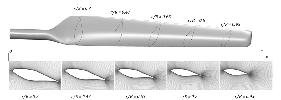
A series of 3D simulations were carried out on five radial positions of the NREL Phase-VI wind turbine, whose geometrical properties are taken from [11] and shown in Table 3. Figure 5 shows the full NREL Phase VI blade and highlights the five analysed sections, highlighting how the chord length, angle of attack and twist angle decrease as the blade radius increases, leading to different flow regimes along the entirety of the blade’s span. The chosen wind speed V is equal to 7 m/s and the relative velocity Vr is found from Eq. 17:

Table 3: Geometrical properties and experienced velocity of the five sections.
|
r/R |
c [m] |
Vr [m/s] |
ω [rpm] |
α [°] |
ϑ [°] |
|
0.3 |
0.711 |
13.35 |
72 |
14.31 |
17.29 |
|
0.47 |
0.627 |
19.14 |
72 |
13.73 |
7.71 |
|
0.63 |
0.543 |
24.89 |
72 |
12.18 |
4.15 |
|
0.8 |
0.457 |
31.13 |
72 |
10.38 |
2.62 |
|
0.95 |
0.381 |
36.69 |
72 |
9.47 |
1.53 |
When present, the jet velocity is assigned so that the coefficient of jet momentum is Cµ = 0.004; 0.008; 0.012, which is defined as:
where Uj and Aj are the jet’s velocity and exit area, respectively, while Utip and Aref are the velocity at the blade's tip and reference planform area. The jet’s thickness varies with the radial coordinate r but follows the same ratio tj/c = 0.2%. The power Pj required to operate the jet is estimated from Eq. 19, assuming a compression efficiency ηc = 0.85. The power percentage change is determined from Eq. 20:

Computed torque and power are reported in Table 4.
Table 4: Computed torque, power and experimental data.
|
|
T [Nm] |
Pnet [kW] |
|
|
Experiment [11] |
803.6 |
6.06 |
/ |
|
Baseline |
963.5 |
7.26 |
/ |
|
Cμ = 0.004 |
1094.1 |
8.02 |
+9.7 |
|
Cμ = 0.008 |
1266.8 |
8.75 |
+19.7 |
|
Cμ = 0.012 |
1408.1 |
9.14 |
+25.1 |
Due to its limitations, it is evident that BEM overestimates the parameters of interest; however, some interesting remarks can still be made. Implementation of the Coanda technology improved power generation by a margin of 25.1% thanks to a substantial increase in lift force coupled with a slight increase in drag force, typical of jet blowing. This aspect is highlighted in Figure 6, where the pressure coefficients CP of the five tested sections are shown for the baseline and jet-on configurations.
Figure 6a displays the CP of the section closer to the blade’s root: the jet amplifies the area between the two curves. However, this effect is mostly located near the trailing edge area for the lowest tested Cµ; but with its increase, an evident upward shift of the suction side curve is achieved, caused by the higher suction at the impingement point, showing the jet’s capability of influencing the whole flow field across the blade, justifying the improvement of lift force. In the sections at r/R = 0.47 (Figure 6b) and r/R = 0.63 (Figure 6c), it can be observed that the increase in the area enclosed by the two curves is more uniform across all tested cases but becomes increasingly pronounced as Cµ increases. From this point onward (Figure 6d and Figure 6e), the baseline curves of both suction and pressure side overlap with their jet-on counterparts, with the exception of the Cµ = 0.012 cases in the r/R = 0.8 section due to the higher jet velocity, suggesting an almost negligible response to the injected pressurised flow. This can be explained by the increase of relative velocity in the sections closer to the blade’s tip, which becomes increasingly similar to the jet’s velocity, diminishing the difference in momentum between the two, hence flow deflection.
Figure 7 further clarifies the aforementioned conclusion: it is evident that for both the torque coefficient (a) and the thrust coefficient (b), the most significant portion of the increase is located from the mid-span toward the blade root, thanks to the large contribution of the induced lift force from the circulation control technique.
Saturation is quickly reached from mid-span onward as there are no noticeable increases in lift force, as already shown in the CP plots proposed in Fig. 6.
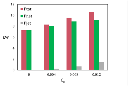
Figure 8 shows the total and net power output and the power expended to operate the jet. This figure highlights the energy efficiency of the blowing jet technology, as an increase in net power is observed for all tested cases; it is noticeable that the energy expenditure for the jet increases rapidly due to its dependence on the cube of the slot exit velocity, as shown in Eq. 19. In fact, even if a net positive output is achieved for all the tested cases, Figure 9 clearly indicates a plateau in net percentage gain in proximity of the last employed Cµ (i.e. vj = 65.3 m/s). Thus, it is evident that the jet’s velocity cannot be indefinitely augmented for a fixed wind speed. As an example, an increase of one order of magnitude of the jet’s velocity would, in turn, translate to a power expense a thousand times greater.
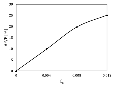
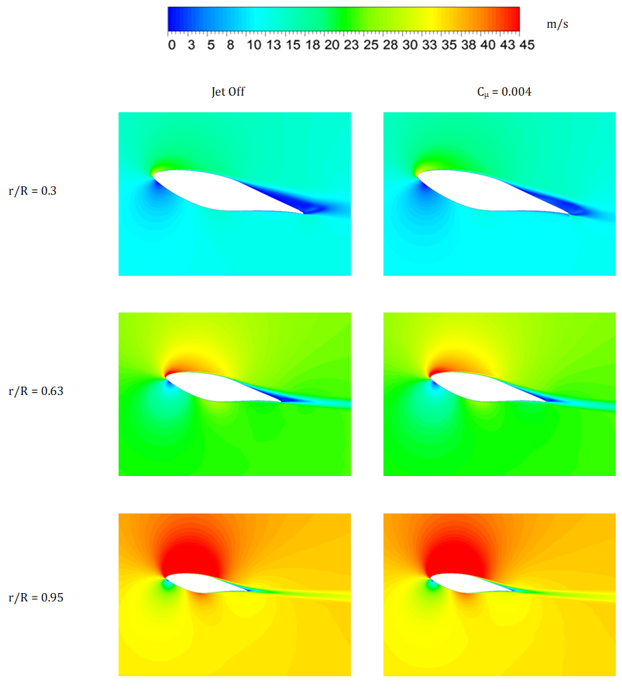
Figure 10 shows the contours of the time-averaged velocity for the innermost, mid-span and blade’s tip sections for the jet-off (left column) and the Cµ = 0.004 configurations (right column). Three main differences can be noticed in the first row: first, in the jet-on configuration, there is an increase in peak velocity at the leading edge of the airfoil; second, a bigger high-velocity area on the suction side is found and lastly the recirculation bubble decreases in size and the wake appears to be rotated by a couple of degrees, which justifies, in fact, the increment in lift force according to Kutta-Žukovskij’s theorem, and these considerations remain noticeable for the second row (i.e. the mid-span section). Once the blade’s tip is reached (third column), however, the jet loses effectiveness. This result suggests that the same increase in power output can be obtained by placing the jet only up to the middle of the blade’s radius.
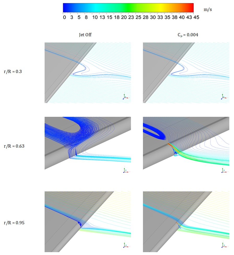
Lastly, the velocity streamlines on the mid-plane of the three sections above are shown in Figure 11. For the r/R = 0.3 section, the jet suppresses the trailing vortex in favour of a more ordered flow field. Additionally, velocity streamlines appear to be more inclined compared to the jet-off counterpart. The recirculation bubble on section r/R = 0.63 drastically decreases in size, and the streamlines follow the trailing edge curvature. In the r/R= 0.95 section, no difference is found between the two cases.
4. Conclusions
A 3D Delayed Detached Eddy Simulation campaign has been conducted on a series of sections along the blade, based on the S809 airfoil, of the NREL Phase-VI wind turbine. The work aimed to show how the injection of a pressurised flow near the airfoil’s leading edge (x/c = 0.95) would increase its performance and, most importantly, assess the energy efficiency of the proposed technology.
The section at 75% of the blade radius was first simulated and results were confronted with Somer’s [10] for mesh validation. Then, the five radial positions along the blade on which experimental values are available from the NREL experimental campaign [11] were simulated, considering the variation of chord length, twist angle and angle of attack.
The power generated was estimated via Blade Element Momentum theory. Three different values of the jet momentum coefficient were considered, namely Cµ = 0.004; 0.008; 0.012. Results have shown how this technology improves the turbine power output up to 25.1% for the highest studied value of the Cµ at very little expense for the chosen wind speed of 7 m/s, which was kept constant throughout all the simulations. The most substantial variations were found near the blade root and in the middle sections, however, suggesting the employment of the proposed technique only for those sections, at least for a fixed Cµ. Moreover, the results showed that the increase in net power can reach a plateau, after which a decrease will inevitably follow due to the excessive energy consumed by the jet which, as mentioned above, depends on the cube of its velocity. Future developments might include the introduction of different slots along the blade with varying momentum (i.e. modulating velocity) to fully exploit the jet along the whole rotor radius, further improving performances.
References
[1] International Energy Association. (2023, June). [Online]. Available: View Article
[2] World Wind Energy Association. (2023, 7 November). [Online]. Available:
View Article
[3] REN21. 2023. Renewables 2023 Global Status Report collection, Renewables in Energy Supply
[4] R. J. Englar, "Circulation Control for High Lift and Drag Generation on STOL Aircraft," Journal of Aircraft, vol. 12, no. 5, pp. 457-463, May 1975.
View Article
[5] H. Djojodihardjo, M. F. Abdul Hamid, A. A. Jaafar, S. Basri, F. I. Romli, F. Mustapha, A. S. Mohd Rafie and D. L. A. Abdul Majid, "Computational Study on the Aerodynamic Performance of Wind Turbine Airfoil Fitted with Coandă Jet," Journal of Renewable Energy, vol. 2013, pp. 1-17, 2013.
View Article
[6] D. Greenblatt and I. J. Wygnanski, "The control of flow separation by periodic excitation," Progress in Aerospace Sciences, vol. 36, no. 7, pp. 487-545, Oct. 2000.
View Article
[7] Hanns Müller-Vahl, Christian Navid Nayeri, Christian Oliver Paschereit, and D. Greenblatt, "Dynamic stall control via adaptive blowing,"Renewable Energy, vol. 97, pp. 47-64, Nov. 2016.
View Article
[8] J. Anderson, Introduction to Flight. New York, Ny: Mcgraw-Hill Education, 2016.
[9] R. J. Englar, "Circulation control pneumatic aerodynamics: blown force and moment augmentation and modification - Past, present and future," Fluids 2000 Conference and Exhibit, Jun. 2000, doi: https://doi.org/10.2514/6.2000-2541. View Article
[10] D. M. Somers, Design and Experimental Results for the S809 Airfoil. 1997.
View Article
[11] M.M. Hand, D.A. Simms, L.J. Fingersh, D.W. Jager, J.R. Cotrell, S. Schreck and S.M. Larwood, "Unsteady Aerodynamics Experiment Phase VI: Wind Tunnel Test Configurations and Available Data Campaigns," Dec. 2001, doi: https://doi.org/10.2172/15000240.
View Article
[12] I. Petracci, L. Manni, M. Angelino, S. Corasaniti, F. Gori, "A 2d-Numerical Study on Slot Jet Applied to a Wind Turbine as a Circulation Control Technique", XII International Conference on Computational Heat, Mass and Momentum Transfer, Series: E3S Web of Conferences Volume 128 (2019), Editor: Mohamad, A. Jan Taler, Ali Cemal Benim EDP Sciences, 2019. , ISBN: 9781510898547
[13] G. Tosatti, L. Manni, and I. Petracci, "A 3D-DDES Numerical Simulation of Jet Blowing as a Power Enhancement Technique Applied to a Wind Turbine with S809 Profile," Proceedings of the World Congress on Mechanical, Chemical, and Material Engineering, Aug. 2024, doi: https://doi.org/10.11159/htff24.136.
View Article
[14] A. N. Kolmogorov, "A refinement of previous hypotheses concerning the local structure of turbulence in a viscous incompressible fluid at high Reynolds number," Journal of Fluid Mechanics, vol. 13, no. 1, pp. 82-85, May 1962, doi: https://doi.org/10.1017/s0022112062000518.
View Article
[15] P. R. Spalart, "Comments on the feasibility of LES for wings, and on a hybrid RANS/LES approach," Jan. 1997.
[16] J. SMAGORINSKY, "GENERAL CIRCULATION EXPERIMENTS WITH THE PRIMITIVE EQUATIONS," Monthly Weather Review, vol. 91, no. 3, pp. 99-164, Mar. 1963, doi: https://doi.org/10.1175/1520-0493(1963)091%3C0099:GCEWTP%3E2.3.CO;2.
View Article
[17] F. R. Menter, M. Kuntz and R. Langtry, "Ten Years of Industrial Experience with the SST Turbulence Model," Proceedings of the 4th International Symposium on Turbulence, Heat and Mass Transfer, Begell House Inc., West Redding, 2003, pp. 625-632.
[18] P. R. Spalart, "Strategies for turbulence modelling and simulations," International Journal of Heat and Fluid Flow, vol. 21, no. 3, pp. 252-263, Jun. 2000, doi: https://doi.org/10.1016/s0142-727x(00)00007-2.
View Article
[19] P. R. Spalart, S. Deck, M. L. Shur, K. D. Squires, M. Kh. Strelets, and A. Travin, "A New Version of Detached-eddy Simulation, Resistant to Ambiguous Grid Densities," Theoretical and Computational Fluid Dynamics, vol. 20, no. 3, pp. 181-195, May 2006, doi: https://doi.org/10.1007/s00162-006-0015-0.
View Article
[20] F. Menter, "Zonal Two Equation k-w Turbulence Models For Aerodynamic Flows," 23rd Fluid Dynamics, Plasmadynamics, and Lasers Conference, Jul. 1993, doi: https://doi.org/10.2514/6.1993-2906.
View Article
[21] Fluent, A. N. S. Y. S. (2011). Ansys fluent theory guide. Ansys Inc., USA, 15317, 724-746
[22] S. V. Patankar. Numerical heat transfer and fluid flow. Series in computational methods in mechanics and thermal sciences. Hemisphere Publ. Co, New York, 1980.
[23] K. Duraisamy, W. J. McCroskey, and J. D. Baeder, "Analysis of Wind Tunnel Wall Interference Effects on Subsonic Unsteady Airfoil Flows," Journal of Aircraft, vol. 44, no. 5, pp. 1683-1690, Sep. 2007. View Article
[1] International Energy Association. (2023, June). [Online]. Available: View Article
[2] World Wind Energy Association. (2023, 7 November). [Online]. Available: View Article
[3] REN21. 2023. Renewables 2023 Global Status Report collection, Renewables in Energy Supply
[4] R. J. Englar, "Circulation Control for High Lift and Drag Generation on STOL Aircraft," Journal of Aircraft, vol. 12, no. 5, pp. 457-463, May 1975. View Article
[5] H. Djojodihardjo, M. F. Abdul Hamid, A. A. Jaafar, S. Basri, F. I. Romli, F. Mustapha, A. S. Mohd Rafie and D. L. A. Abdul Majid, "Computational Study on the Aerodynamic Performance of Wind Turbine Airfoil Fitted with Coandă Jet," Journal of Renewable Energy, vol. 2013, pp. 1-17, 2013. View Article
[6] D. Greenblatt and I. J. Wygnanski, "The control of flow separation by periodic excitation," Progress in Aerospace Sciences, vol. 36, no. 7, pp. 487-545, Oct. 2000. View Article
[7] Hanns Müller-Vahl, Christian Navid Nayeri, Christian Oliver Paschereit, and D. Greenblatt, "Dynamic stall control via adaptive blowing,"Renewable Energy, vol. 97, pp. 47-64, Nov. 2016. View Article
[8] J. Anderson, Introduction to Flight. New York, Ny: Mcgraw-Hill Education, 2016.
[9] R. J. Englar, "Circulation control pneumatic aerodynamics: blown force and moment augmentation and modification - Past, present and future," Fluids 2000 Conference and Exhibit, Jun. 2000, doi: https://doi.org/10.2514/6.2000-2541. View Article
[10] D. M. Somers, Design and Experimental Results for the S809 Airfoil. 1997. View Article
[11] M.M. Hand, D.A. Simms, L.J. Fingersh, D.W. Jager, J.R. Cotrell, S. Schreck and S.M. Larwood, "Unsteady Aerodynamics Experiment Phase VI: Wind Tunnel Test Configurations and Available Data Campaigns," Dec. 2001, doi: https://doi.org/10.2172/15000240. View Article
[12] I. Petracci, L. Manni, M. Angelino, S. Corasaniti, F. Gori, "A 2d-Numerical Study on Slot Jet Applied to a Wind Turbine as a Circulation Control Technique", XII International Conference on Computational Heat, Mass and Momentum Transfer, Series: E3S Web of Conferences Volume 128 (2019), Editor: Mohamad, A. Jan Taler, Ali Cemal Benim EDP Sciences, 2019. , ISBN: 9781510898547
[13] G. Tosatti, L. Manni, and I. Petracci, "A 3D-DDES Numerical Simulation of Jet Blowing as a Power Enhancement Technique Applied to a Wind Turbine with S809 Profile," Proceedings of the World Congress on Mechanical, Chemical, and Material Engineering, Aug. 2024, doi: https://doi.org/10.11159/htff24.136. View Article
[14] A. N. Kolmogorov, "A refinement of previous hypotheses concerning the local structure of turbulence in a viscous incompressible fluid at high Reynolds number," Journal of Fluid Mechanics, vol. 13, no. 1, pp. 82-85, May 1962, doi: https://doi.org/10.1017/s0022112062000518. View Article
[15] P. R. Spalart, "Comments on the feasibility of LES for wings, and on a hybrid RANS/LES approach," Jan. 1997.
[16] J. SMAGORINSKY, "GENERAL CIRCULATION EXPERIMENTS WITH THE PRIMITIVE EQUATIONS," Monthly Weather Review, vol. 91, no. 3, pp. 99-164, Mar. 1963, doi: https://doi.org/10.1175/1520-0493(1963)091%3C0099:GCEWTP%3E2.3.CO;2. View Article
[17] F. R. Menter, M. Kuntz and R. Langtry, "Ten Years of Industrial Experience with the SST Turbulence Model," Proceedings of the 4th International Symposium on Turbulence, Heat and Mass Transfer, Begell House Inc., West Redding, 2003, pp. 625-632.
[18] P. R. Spalart, "Strategies for turbulence modelling and simulations," International Journal of Heat and Fluid Flow, vol. 21, no. 3, pp. 252-263, Jun. 2000, doi: https://doi.org/10.1016/s0142-727x(00)00007-2. View Article
[19] P. R. Spalart, S. Deck, M. L. Shur, K. D. Squires, M. Kh. Strelets, and A. Travin, "A New Version of Detached-eddy Simulation, Resistant to Ambiguous Grid Densities," Theoretical and Computational Fluid Dynamics, vol. 20, no. 3, pp. 181-195, May 2006, doi: https://doi.org/10.1007/s00162-006-0015-0. View Article
[20] F. Menter, "Zonal Two Equation k-w Turbulence Models For Aerodynamic Flows," 23rd Fluid Dynamics, Plasmadynamics, and Lasers Conference, Jul. 1993, doi: https://doi.org/10.2514/6.1993-2906. View Article
[21] Fluent, A. N. S. Y. S. (2011). Ansys fluent theory guide. Ansys Inc., USA, 15317, 724-746
[22] S. V. Patankar. Numerical heat transfer and fluid flow. Series in computational methods in mechanics and thermal sciences. Hemisphere Publ. Co, New York, 1980.
[23] K. Duraisamy, W. J. McCroskey, and J. D. Baeder, "Analysis of Wind Tunnel Wall Interference Effects on Subsonic Unsteady Airfoil Flows," Journal of Aircraft, vol. 44, no. 5, pp. 1683-1690, Sep. 2007. View Article