Journal of Fluid Flow, Heat and Mass Transfer (JFFHMT)

ISSN: 2368-6111

1. Introduction

A hygienic hospital operating room determines human life or death; thus, it needs particular concern. A study [1] shows that 5 to 10 percent of patients in acute care hospitals acquire one or more infections. This adverse event affects approximately 2 million patients annually in the United States, results in about 90,000 deaths, and adds an estimated $4.5 to $5.7 billion per year to the costs of patient care.

All the danger in operating rooms comes from the contaminants. Unfortunately, sterilization alone cannot remove it because of their propagation from the patient's wound. Many studies have shown that a very effective method to remove contaminants is driving them out by the conditioned air. Thus, operating rooms require ventilation and air conditioning to achieve thermal comfort and remove contaminants.

The design of an HVAC system for an operating room is built on many factors besides cooling load, beginning from the room structure, lights and surgeon's positions, equipment layout, and even the surgeon's movement. These factors make it hard to design an optimum system, and conducting experimental studies will be even more challenging because the work requires too many diffuser locations and sizes. Therefore, numerical simulation, which depends merely on computational fluid dynamics (CFD), is the more appropriate method for achieving this.

2. Related Work

The increasing developments of computational fluid dynamics in recent years have opened the possibilities for improving HVAC systems in the design phase, with fewer experiments required, yielding low-cost yet effective systems [2]. One can apply CFD modelling and simulation to provide valuable indications on proper indoor microclimate conditions and IAQ (Indoor Air Quality) by examining the effectiveness and efficiency of various HVAC systems through quickly changing the location of diffusers, supply air conditions, and system control schedules [3].

According to the ASHRAE Applications Handbook [4], the temperature in the operating room (OR) should be in the range of 68–76F (20–24C), and the relative humidity should be between 50% and 60%, and these are semi-agreed with AIA guidelines (20-23C) and (45%-55%). ASHRAE and AIA state that positive air pressure should be maintained, and all air exhausted with no recirculation is preferred [5]. The National Institute of Health (NIH) research has shown that 20 air changes per hour (ACH) are optimal for a general-purpose operating room. They sometimes specify higher air change rates for ORs where higher-risk procedures occur. Balocco et al. [3] confirmed the strong effects of a correct ventilation system design and location of the air supply diffusers on compliance with microclimatic conditions, IAQ levels, and satisfactory contaminant removal. Essam E. Khalil [6] recommended using a laminar diffuser as it achieved driving contaminants from the operating room. At the same time, Yunlong Liu et al. [7] asserted that operating with a 6-lamp light and a centre table under the laminar diffuser resulted in 100% particle displacement efficiency.

Memarzadeh and Manning [8] mentioned that a care needs to be taken in the sizing of the laminar flow array. A face velocity of around 30 to 35 fpm (0.15 to 0.18 m/s) is sufficient from the laminar diffuser array, that the array size itself should be set correctly.

3. Mathematical Equations

Numerical simulation determines the efficient air conditioning system by solving the governing equations (in the discretized form) for the conservation of mass (continuity), momentum (Nervier-Stokes equations), energy, and species transport equations. In a Cartesian coordinate system.

3. 1. The Mass Conservation Equation

Assuming that the flow is incompressible; thus, the mass conservation equation in the steady-state condition is presented in Eq. 1 as:

(1)

Where V is the velocity vector of air, u,v and w are the velocity components (m/s) in the x, y, and z directions, respectively.

3. 2. The Momentum Conservation Equation

For incompressible flow, the general form of the momentum conservation equation is presented in Eq. 2 as:

(2)

Where ρ is the air density (kg/m³),  is as defined above, ρ is the air pressure (N/m²), μ is the air viscosity (kg/m. s), f is the body force (gravity) (N/m³)

3. 3. The Energy Conservation Equation

Assuming that the thermal conductivity is scalar, with no heat generation, the simplified energy conservation equation (Eq. 3) becomes:

(3)

Where ρ is the air density (kg/m3), c_p is specific heat of air (J/ (kg. K)), V is as defined above, T is temperature (K) and k is thermal conductivity of air (W/ (m K)).

3. 4. Species Transport Equation

Assuming that the mass diffusivities of species in the airflow are scalars, thermal diffusion is negligible, and there is no chemical reaction, the species transport equation (Eq.4) is given by:

(4)

Where D is the mass diffusivity of species in air (m²/s), C is the mean species concentration (kg/kg mixture) and U is the velocity vector of the mixture.

Using ANSYS Fluent these equations are solved (in FVM discretization form) with the two realizable k-ɛ model equations which consists of kinetic energy equation and turbulent dissipation rate equation (Eq. 5 and Eq. 6) mentioned respectively:

3. 5. The Kinetic Energy Equation (k)

(5)

3. 6. The Turbulent Dissipation Rate Equation (ɛ)

(5)

Where ρ and V are as defined above, ε is the dissipation rate of turbulent kinetic energy, μ_t is the turbulent kinetic energy (m²/s²), μ_t is the turbulent viscosity (kg/m. s), σ_k and σ_ε are the turbulent Prandtl numbers for k and ε respectively, is the production of turbulent kinetic energy (kg/m.s³), G_b is the buoyancy production term (kg/m.s3). S_k and S_ε are user-defined source terms. C₁, C₂, and C₃ are model constants, typically determined empirically.

The design of OR requires rigorous work to achieve thermal comfort and contaminant removal. Inside the operating room, all fluid properties, including temperature, velocity, pressure, relative humidity, and contaminant removal, must be assessed using the mentioned governing equations for the various air conditioning schemes to determine the most efficient one.

Table 1. Boundary Conditions

NO.	Entity	Temperature/ Heat Flux	Dimensions (m)
1	Inlet	15 C	Variable
2	EDL Surgical Lights (face)	210.122 W/m2	0.47 X 0.42 X 0.15
3	EDL Surgical Lights (back)	10.506 W/m2
4	Fluorescent Lamps	200 W/m2	0.6 X 0.6
5	Wall	20.8274 W/m2	5 X 3
6	Roof	214.868 W/m2	5 x 5
7	Floor	29.05 W/m2
8	Surgical Unit	282.6 W/m2	0.46 X 0.51 X 1.01
9	Anaesthesia Machine	14.02 W/m2	0.4 X 0.47 X 1.45
10	Surgeon	49.612 W/m2	0.25 X 0,25 X 1.55
11	Patient Skin	91.263 W/m2	0.12 X 0.16 X 1.35
12	Patient Wound	91.263 W/m2

4. Cooling Load Calculation

Table 1 illustrates objects dimensions and the heat fluxes inside the operating room.

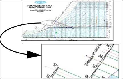
The velocity and temperature are found after estimating the cooling load (13.210 kW) using a psychrometric chart, as in Figure 1. Noting that the patient's stomach, is considered a contaminant source.

The Contaminants removal effectiveness (CRE) estimation is also included in this research. It is defined as the ratio between the concentration of contaminants at the exhaust point and the mean value of contaminant concentration within a specific zone. Its simplified equation (Eq.7) is defined as follows [9]:

(7)

Where C_E is the contaminants concentration in the exhaust while C_zj is the contaminant concentration in a specific zone, assuming that the contaminants concentration in the inlet diffuser equals zero.

In order to achieve the human thermal comfort, the total air supply is calculated using the psychrometric chart and it equals 37 ACH with outdoor air changes equal to 7 ACH which is around 19% of the total air changes. This percent is similar to ASHRAE recommendation of that the fresh air must be 20% from total air supply [10].

5. Simulation Procedure

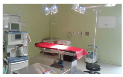
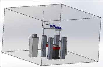
A real room with dimensions 5m×5m×3m (illustrated in Figure 2) is modelled using SolidWorks and simulated using ANSYS Fluent to achieve thermal comfort and contaminant removal.

5.1. Validation of Results

Before implementing the simulation for the current model, the setup was validated using a previous study conducted by [11]. This study involved both experimental and numerical analyses of airflow in a surgical room. The experimental analysis assessed environmental conditions, specifically temperature and velocity, at four points (B, C, D, and E) in the surgical room, with sensors positioned at two heights (0.6m and 1.2m) on each pedestal as seen in Figure 3. [11] found a strong correlation between the simulation and experimental results. Consequently, the current study applies the same geometry, and boundary conditions as [11] but with a different setup procedure that includes a different turbulence model (realizable k-ɛ model), in order to compare the present numerical results (S2) with the numerical and experimental data (S1 and E1, respectively) from [11]. The results of the comparisons of velocity and temperature are shown in Tables 2 and 3.

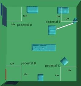
Table 2(a): Velocity at point B

Velocity at point B
Height	0.60 m	1.21 m
Measured	0.41 m/s	0.23 m/s
Simulated [11]	0.08 m/s	0.15 m/s
Simulated (Present)	0.23 m/s	0.26 m/s

 

Table 2(b): Velocity at point C

Velocity at point C
Height	0.60 m	1.21 m
Measured	0.31 m/s	0.21 m/s
Simulated [11]	0.19 m/s	0.09 m/s
Simulated (Present)	0.41 m/s	0.21 m/s

Table 2(c): Velocity at point D

Velocity at point D
Height	0.60 m	1.21 m
Measured	0.37 m/s	0.23 m/s
Simulated [11]	0.26 m/s	0.16 m/s
Simulated (Present)	0.23 m/s	0.17 m/s

Table 2(d): Velocity at point E

Velocity at point E
Height	0.60 m	1.21 m
Measured	0.14 m/s	0.31 m/s
Simulated [11]	0.51 m/s	0.18 m/s
Simulated (Present)	0.17 m/s	0.41 m/s

5.1. 2. Temperature Comparison

Table 3(a): Temperature at point B

Temperature at point B
Height	0.60 m	1.21 m
Measured	18.5 ºC	18.8 ºC
Simulated [11]	18.3 ºC	18.4 ºC
Simulated (Present)	17.9 ºC	17.9 ºC

 

Table 3(b): Temperature at point C

Temperature at point C
Height	0.60 m	1.21 m
Measured	18.7 ºC	19.4 ºC
Simulated [11]	18.3 ºC	18.3 ºC
Simulated (Present)	17.9 ºC	18 ºC

 Table 3(c): Temperature at point D

Temperature at point D
Height	0.60 m	1.21 m
Measured	19.4 ºC	18.9 ºC
Simulated [11]	18.3 ºC	18.4 ºC
Simulated (Present)	17.8 ºC	17.9 ºC

Table 3(d): Temperature at point E

Temperature at point E
Height	0.60 m	1.21 m
Measured	18.0 ºC	18.3 ºC
Simulated [11]	18.2 ºC	18.3 ºC
Simulated (Present)	17.8 ºC	17.9 ºC

From the velocity comparison tables (tables 2), it can be seen clearly that the new setup procedures are more accurate and robust than the results of [11]. This is due to the use of realizable k-ɛ model, which is better in terms of boundary flows than the standard k-ɛ model that was used by [11].

The temperature comparison tables (tables 3) show that the temperature results for most of the points is better for [11] than the new setup procedure, but still the deviation from the experimental results for the current model is maximumly equal 8% at Point D (0.6 m height ) which is an acceptable deviation if compared with [11] results which has a maximum deviation of 6% at point C (1.21 m height).

5. 2. Geometry

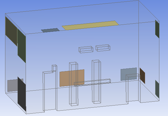
The 3D model of the room is presented in Figure 4 and due to the complexity of the geometry, which results in low-quality mesh, thus convergence problems, the geometry was simplified using symmetry plane which results in using less computational power. Figure 5 shows the simplified model.

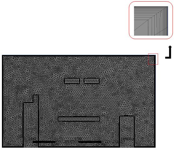
5. 3. Mesh Independence Study

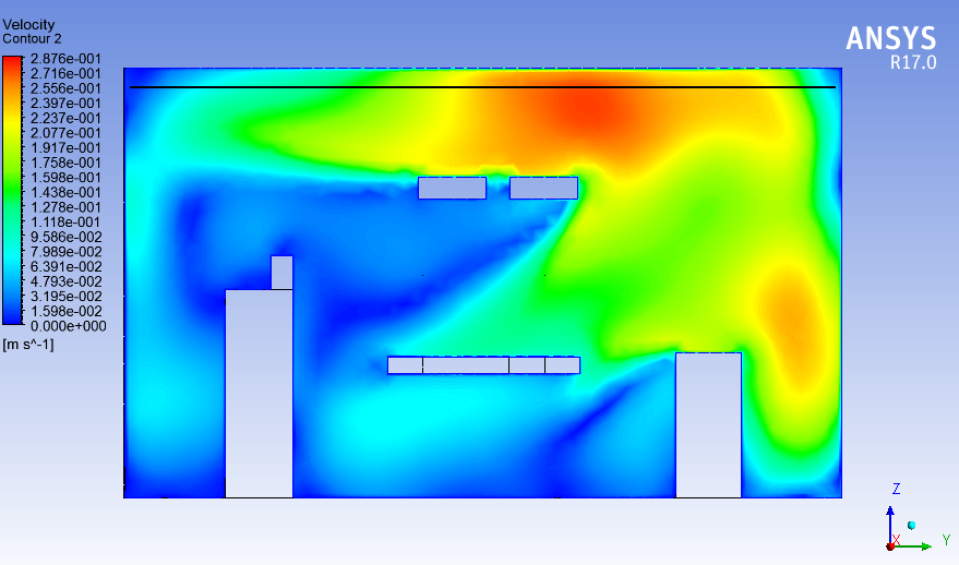
In the present case study, five meshes with different element sizes, 321,000, 620,000, 902,000, 1,350,000, and 2,048,000 elements, are investigated to identify the minimum mesh density to ensure that the converged solution obtained from CFD is independent of the mesh resolution. Velocity contours are used for comparing the performance of different mesh sizes by a horizontal line drawn across the room. The line location is selected in the most variant velocity contour in the y-direction (See Figure 6(a)). The results are in Figure 6(b)

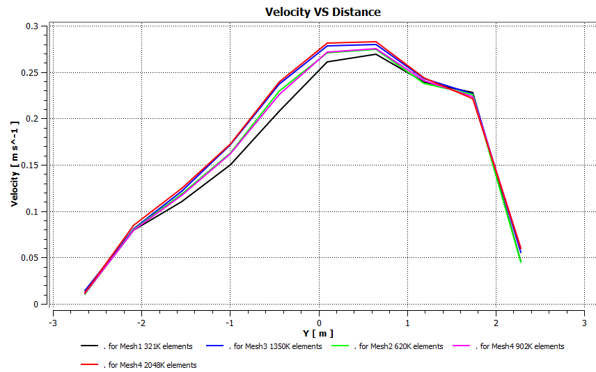
Based on the above, a mesh with 1,350,000 elements (see Figure. 6(b) and Figure. (7)) is sufficient to carry out the simulation, as it gives a mesh-independent result at the minimum possible computational cost and time.

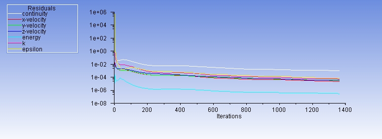
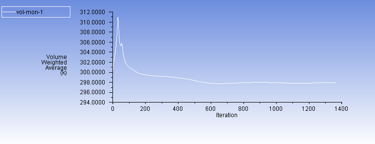
5. 4. Examination of Convergence Criteria

In order to verify that the solution is insensitive to the error, three convergence criteria are used. The first is mass balance which is tested by measuring the mass flow rate at both inlet and outlet and it’s found that the value is equal for both (0.459 kg/s).

The other two criteria are Residuals stability and Average static temperature stability which are shown in Figure. 8(a), 8(b):

6. Results and Discussion:

One plane and two zones are used to show the results. The plane is drawn across the patient and is identical to the plane of symmetry (See Figure. 9(a)) and is used to present the results for the patient, Surgical lights and the surgical equipment. velocity vectors, temperature contours and contaminants concentration are presented in this plane. The two zones (Figure 9(b), 9(c)) are used to measure the mean values of the previous characteristics in the overall room (OA) and the occupied zone (OZ) which contains the patient, the surgeons, the surgical lights and the surgical equipment. These mean values are presented in Table 5.

Four main Cases are studied in this research. Their layouts are mentioned in table 4.

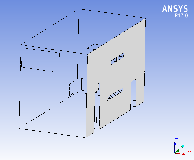
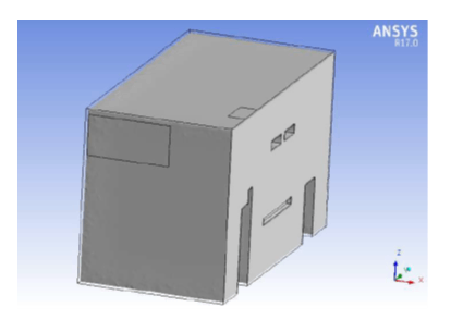
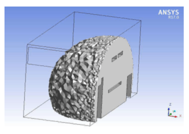
Table 4: Air outlet(s) dimensions, velocity and arrangement

Case No:	Diffuser         Area, ()	Supply Velocity, (m/s)	Arrangement
1	0.7 X 1.4	0.3826	Two upper-sidewall supply grilles, with two lower exhaust grilles in the opposite walls.
2	2 X 1	0.3826	One upper side wall (central horizontally) supply grille with one lower central exhaust grille on the opposite wall.
3	2 X 1	0.3826	One central supply diffuser in the ceiling, with two lower central exhaust grilles
4	2 X 1	0.3826	Case 4 represents one central supply diffuser in the ceiling, with four lower exhaust grilles

Table 5: The Mean Characteristics in Multiple Zones

Case	Air Velocity, m/s		Temperature,		Relative humidity,	CRE
	OA	OZ	OA	OZ	OA	OZ
Case 1	0.14	0.07	30.9	36.9	38.5	0.21
Case 2	0.16	0.10	29.0	29.3	41.5	0.30
Case 3	0.12	0.17	30.1	19.9	50.8	0.40
Case 4	0.10	0.16	35.8	20.6	45.2	0.32

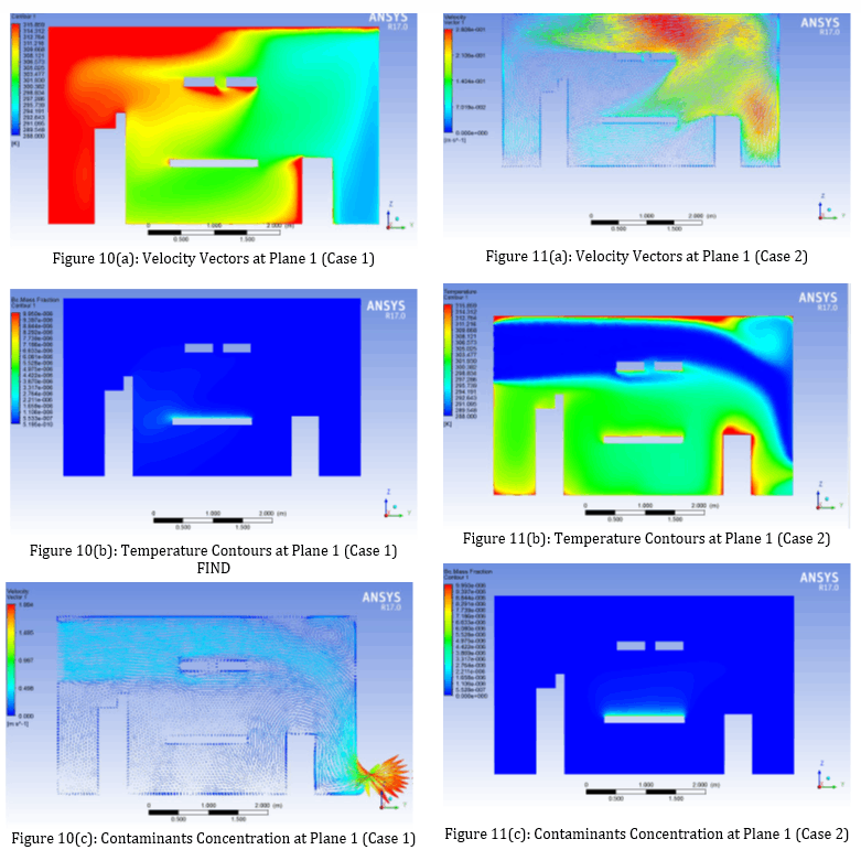
For Case 1 and Case 2, from Figure 10(a) and 11(a) where the side wall diffusers are located respectively in the top corner and centre of the left wall, the velocity vectors for Case 1 at plane 1 (symmetry plane) are distributed with low velocity values comparing to Case 2 where the velocity vectors have a reasonable values which lead the temperature contours to reach the occupied zone in Case 2 (Figure 11(b)) and has lower effect in case 1 (Figure 10(b)), this happened because in Case 1 the exhaust grill (outlet) is located in the bottom corner of the right wall which let most of the conditioned air exit without reaching the occupied zone, on the other hand case 2 where the inlet diffuser is located in the top centre of the left wall and the outlet is symmetrical in the bottom of the right wall will allow the conditioned air smoothly pass through the occupied zone. These configurations will produce higher contaminant removal effectiveness (CRE) for Case 2 (Figure 11(c)) comparing to Case 1 Figure 10(c) as shown in table 5.

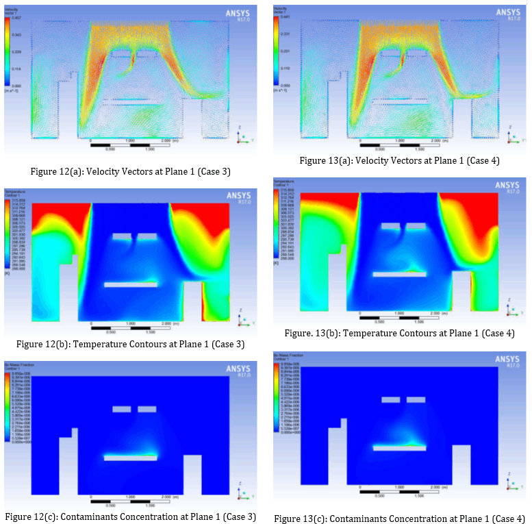
In Case 3 and Case 4, where laminar diffusers are used, It can be noticed from the velocity vectors in Figure 12(a) and Figure 13(a) that the air velocity around the patient is not high and this is due to the obstruction of the surgical lights, but still the airflow in the occupied zone is laminar, with low circulations formed (especially for Case 3), proved by the average velocity values in the occupied zone in Table 5 (0.17 m/s and 0.16 m/s respectively) which falls in the laminar velocity range [8]. Therefore, as mentioned by [6] that this laminar flow can wash more contaminants from the occupied zone.

For temperature contours, it can be noticed for both cases (Case 3, Case 4) that the highest temperatures come from the ceiling, and this is due to the high heat flux which was selected based on the location of the room in the building and the temperature ranges in the country by considering the worst case. Despite that the average temperature in the occupied zone for both cases is about 20℃ as in Table 5, and it is noticed that the temperature at the head of the patient is a little relatively high (Figure 12(b), Figure 13(b)) due to the obstruction of the surgical lights which will result in that more air will exit from the left grills than the right one as can be seen in the velocity vectors (Figure 12(a),Figure 13(a) ). However, it is still normal (25℃).

In the contours of contaminants concentration, it can be seen that for both cases (Case 3, Case 4) the contaminants are slightly, relatively high near the patient head as in Figure 12(c) and Figure 13(c) (higher for Case 4) and this is due to the lower airflow at this area as what has been mentioned. Still the concentration is too low (≈ 3x 10^-6 kg/kg air)

The contaminant removal effectiveness (CRE) and average relative humidity for Case 3 are 0.4, 50.8 % as in Table 5 which are better than Case 4 (0.32,45% respectively). It should be noted that Case 3 has the preferable relative humidity [12] and has the highest CRE value compared to the other cases.

7. Conclusion

This paper conducts and presents numerical simulations of airflow, temperature distribution, and contaminant concentration in a hospital operating room. The results show the strong effect of the supply diffuser(s) and outlet grille(s) positions on thermal comfort and contaminant removal.

Our findings suggest that the central laminar diffuser with two central grilles near the floor (Case 3) is the most effective in achieving optimal airflow, temperature distribution, and contaminant removal in the occupied zone. This practical insight can guide the design and layout of hospital operating rooms, ensuring the best possible thermal comfort and contaminant removal. In contrast, the side wall diffusers (Case 1 and Case 2) may not be as effective due to the limited reach of conditioned air to the occupied zone. Similarly, the central diffuser with four grilles near the floor (Case 4) offers good thermal comfort, but Case 3 surpasses it in terms of contaminant removal.

8. Recommendations

The results of this work recommend the following design considerations for the air distribution system to obtain the best thermal comfort and contaminants removal in operating rooms:

• It is clear that further research is needed to fully understand the complex dynamics of hospital operating rooms. Specifically, more CFD work should be done to study the effect of surgical lights' position, the surgical staff's movement, the equipment layout, and the transient phenomena (e.g., door opening). This ongoing research is crucial for continuously improving the design and functionality of hospital operating rooms.
• The side wall diffuser (if used) must have an inclination angle.

References

[1] Bill Drake, "Infection Control in Hospital", a supplement to ASHRAE Journal, June 2006.
[2] Son H. Ho, Luis Rosario, Muhammad M. Rahman, "Three-dimensional analysis for hospital operating room thermal comfort and contaminant removal", Applied Thermal Engineering Journal, available online 13 November 2008 in journal homepage:
View Article
[3] Carla Balocco, Giuseppe Petrone, Giuliano Cammarata, "Numerical Investigation of Different Airflow Schemes in a Real Operating Theatre", Biomedical Science and Engineering Journal, Published Online February 2015 in SciRes. http://www.scirp.org/journal/jbise
[4] ASHRAE Applications Handbook, 2003.
[5] AIA, AIA Guidelines for Design and Construction of Hospitals and Health Care Facilities, The American Institute of Architects, Washington, DC, 2006.
[6] Essam E. Khalil, "Energy Efficient Hospitals Air Conditioning Systems", Open Journal of Energy Efficiency 2012, Published Online June 2012 (http://www.SciRP.org/journal/ojee).
[7] Yunlong Liu, Alfred Moser, Kazuyoshi Harimoto, "Numerical Study of Airborne Particle Transport in an Operating Room", International Journal of Ventilation Volume 2 No.2, 2003.
[8] F. Memarzadeh and A. P. Manning, "Comparison of Operating Room Ventilation Systems in the Protection of The Surgical Site/Discussion," ASHRAE Transactions, Vol. 108, No. 2, 2002, p.
[9] Carla Balocco, Giuseppe Petrone, Giuliano Cammarata, Pietro Vitali, Roberto Albertini, Cesira Pasquarella, "Indoor Air Quality in a Real Operating Theatre under Effective Use Conditions", Biomedical Science and Engineering Journal, Published Online September 2014 in SciRes. http://www.scirp.org/journal/jbise
[10] ASHRAE_HVAC Design Manual for Hospital and Clinics, Second Edition 2013.
[11] Danilo de Moura, Victor Barbosa Felix, Marcelo Luiz Pereira, Arlindo Tribess, "Experimental and numerical analysis of airflow in a surgical room" Copyright © 2007 by ABCM November 5-9, 2007, Brasília.
[12] McQuiston, Parker, Spilter, "Heating Ventilating, and Air Conditioning, Analysis, and Design", 6th Edition, John Wiley & Sons Inc, 2004.
[2] Son H. Ho, Luis Rosario, Muhammad M. Rahman, "Three-dimensional analysis for hospital operating room thermal comfort and contaminant removal", Applied Thermal Engineering Journal, available online 13 November 2008 in journal homepage: View Article
[3] Carla Balocco, Giuseppe Petrone, Giuliano Cammarata, "Numerical Investigation of Different Airflow Schemes in a Real Operating Theatre", Biomedical Science and Engineering Journal, Published Online February 2015 in SciRes. http://www.scirp.org/journal/jbise View Article
[6] Essam E. Khalil, "Energy Efficient Hospitals Air Conditioning Systems", Open Journal of Energy Efficiency 2012, Published Online June 2012 (http://www.SciRP.org/journal/ojee). View Article
[7] Yunlong Liu, Alfred Moser, Kazuyoshi Harimoto, "Numerical Study of Airborne Particle Transport in an Operating Room", International Journal of Ventilation Volume 2 No.2, 2003. View Article
[8] F. Memarzadeh and A. P. Manning, "Comparison of Operating Room Ventilation Systems in the Protection of The Surgical Site/Discussion," ASHRAE Transactions, Vol. 108, No. 2, 2002, p. View Article
[9] Carla Balocco, Giuseppe Petrone, Giuliano Cammarata, Pietro Vitali, Roberto Albertini, Cesira Pasquarella, "Indoor Air Quality in a Real Operating Theatre under Effective Use Conditions", Biomedical Science and Engineering Journal, Published Online September 2014 in SciRes. http://www.scirp.org/journal/jbise View Article