Journal of Fluid Flow, Heat and Mass Transfer (JFFHMT)
ISSN: 2368-6111

Volume 11 - Year 2024 - Pages 168-176
DOI: 10.11159/jffhmt.2024.017
Improving the Accuracy of Detecting Signs of Combustion Instability by Using Anomaly Detection
Koji Maeta1, Takenao Ohkawa 1
1Graduate School of System Informatics, Kobe University
1-1 Rokkodai-Cho Nada-Ku Kobe-City, Hyogo 657-8501, Japan
189x601x@stu.kobe-u.ac.jp;
ohkawa@kobe-u.ac.jp
Abstract - In this paper, a simple combustion device consisting of a premixed burner, a rectangular cylinder, and a visualization window was used to measure the pressure fluctuation level and flame images while varying the flame position and operating conditions. A Convolutional Autoencoder (CAE) was applied to the acquired images to extract the features of the images. The images reconstructed from the extracted features and the original acquired images were then used to define the Combustion Instability Index (ΔCAETI_err), which can be used to quantify the flame conditions. By organizing the correlation between the proposed Combustion Instability Index and the combustion oscillation levels, we evaluated the possibility of detecting signs of increase in the combustion oscillation. The results showed that the proposed Combustion Instability Index and the combustion oscillation level were highly correlated. Using Grad-CAM data analysis, which enables visualization of the Combustion Instability Index on a two-dimensional plane, the mechanism that causes the increase in the combustion oscillation level was discussed by evaluating the effects of operating conditions on the flame distribution.
Keywords: Premixed combustion, Combustion instability, Convolutional Autoencoder, Grad-CAM.
© Copyright 2024 Authors - This is an Open Access article published under the Creative Commons Attribution License terms Creative Commons Attribution License terms. Unrestricted use, distribution, and reproduction in any medium are permitted, provided the original work is properly cited.
Date Received: 2023-09-05
Date Revised: 2024-05-06
Date Accepted: 2024-05-28
Date Published: 2024-07-15
1. Introduction
To improve the reliability of combustors in gas turbines and rocket engines, it is necessary to measure and monitor the operating conditions with various sensors to prevent the occurrence of sudden abnormal conditions. Research has been conducted on a method that can detect signs of combustion instability during lean combustion by measuring pressure fluctuation data inside the combustor and then analysing those data using machine learning and deep neural networks (DNN) [1 - 3].
On the other hand, to determine whether the combustion oscillation level has increased, not only the pressure fluctuation data but also the information about the spatial distribution and time variation of the flame are important. There are a number of studies that investigated the distribution of heating rate fluctuations and flame shape characteristics to identify signs of combustion instability. For example, a method of directly evaluating the heat release rate fluctuations has been proposed, in which OH radicals in a flame are made to fluoresce to visualize and measure their distribution in the flame (OH-PLIF method) [4 - 5]. Research and other activities to monitor and classify combustion conditions and evaluate combustion instability have also been conducted actively in recent years by analysing these image data using machine learning and Convolutional Neural Networks (CNN) [6 - 8].
In this study, combustion experiments were conducted using a simple combustion device consisting of a burner with a swirler nozzle and a rectangular cylinder with a visualization window. Flame images acquired by a High-speed camera were analysed using a Convolutional Autoencoder to extract flame features. The difference between the reconstructed image based on the feature values and the input image was defined as the Combustion Instability Index, and the relationship between this index and the combustion oscillation level was discussed. In the experiment, the combustion oscillation level was measured by a pressure fluctuation sensor, and combustion experiments were conducted for several cases by varying the fuel-air ratio of the premixed LP gas / air mixture.
2. Experiment Summary
2.1. Experimental device and measuring equipment
The experimental device used in this study is shown in Figure 1.
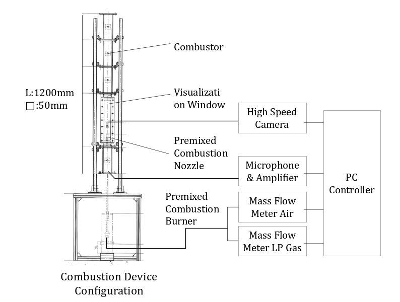
A premixing nozzle with a swirler was inserted into a rectangular cylinder having a square base of 50 mm × 50 mm and a length of 1200 mm, and LP gas (main component: propane) and air was supplied to the nozzle by a mass flow meter (HORIBA: S600-BM212). The combustion oscillation level was measured with a microphone (Bruel & Kjaer: 4938) placed at the combustion cylinder inlet. This microphone can measure sound pressure levels of 30dB (10-3Pa) in the 4-70kHz range. As shown in Figure 3.1(Mentioned later), the maximum sound pressure level was defined as 148dB(410Pa) with a normalized sound pressure level of 1. Therefore, it is possible to measure a Normalized sound pressure level of 10-5 or less. As shown in Figure 3.2, the average value of the normalized sound pressure level under operating conditions with low combustion oscillation levels is on the order of 10-2. It can be said that this experiment has sufficient measurement accuracy. The device used in this study was equipped with a visualization window to observe the flame inside the combustor, and a High-speed camera (FASTCAM: SA3 LCB), capable of measuring monochrome images, was used to take images. The position of the pressure fluctuation resulting from the acoustic mode inside the combustor and the heat release rate fluctuation of the flame are important factors for combustion instability. Since the flame position is intentionally changed during the tests, the position of the visualization window is allowed to move in the flow direction to enable acquisition of the flame images. A Multifunction I/O device (NI: USB-6251) was used to synchronize the mass flow meter, microphone, and High-speed camera outputs. A premixing nozzle with a swirler was used to ensure flame stabilization.
2.2. Experimental conditionWhen obtaining the data under various combustion conditions, the combustion oscillation level and flame image data were obtained by keeping the LP gas flow constant while changing the air flow condition step by step as shown in Table 1.
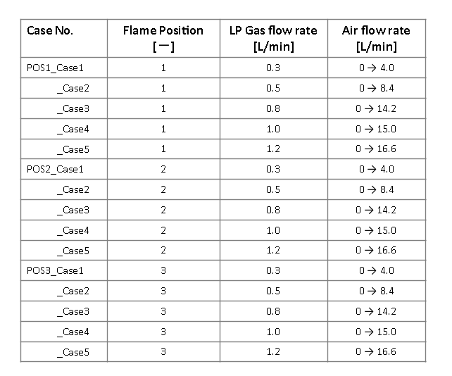
The air flow rate was set to the limit of flame lift and blowout, and the gas flow rate was set to the limit considering the heat resistance of the nozzle (uncooled). As shown on the left of Figure 2, the nozzle was positioned at L/2, L/4, and L/8 from the bottom (upstream) end of the cylinder relative to the total length of the combustion cylinder (L).
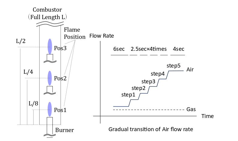
The flame position was varied in order to investigate the effect of the relationship between the antinode, node, and midpoint of the first-order acoustic mode generated in the combustor and the location of the flame on the level of combustion oscillation. The air flow rate was controlled sequentially as shown on the right of Figure 2.
2.3. Equipment Characteristics
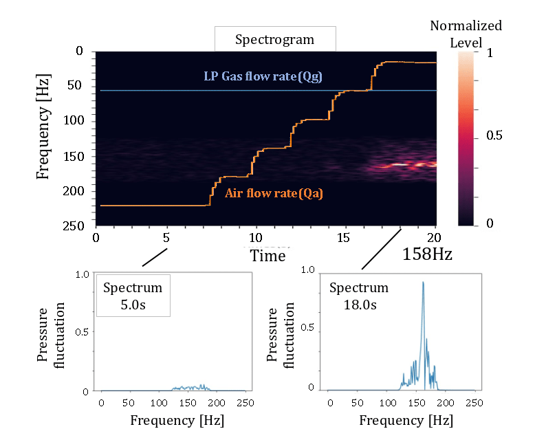
An example of the measurement data obtained from the combustion experiment is shown in Figure 3.1.
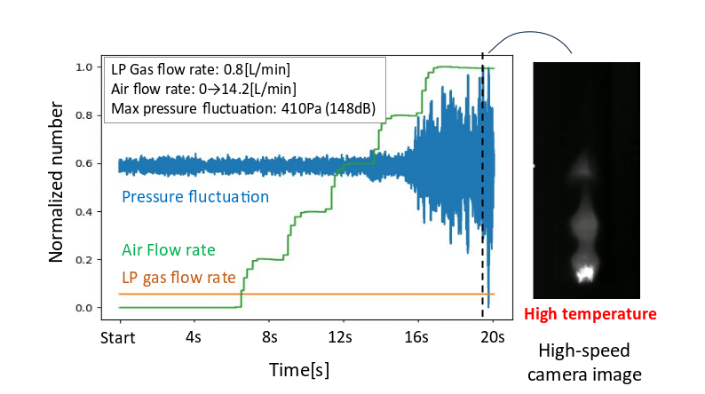
When the air flow rate was increased stepwise after an elapse of 7 seconds after starting the combustion operation sequence, the combustion oscillation level tended to increase gradually as the air flow rate increased. The maximum combustion oscillation level occurred approximately 20 seconds after the start of the step change in air flow rate. The flame image taken by the High-speed camera (19 seconds after the start of the sequence) is shown on the right of Figure 3.1. In the early period after the start of the combustion operation sequence, the air flow rate is low, resulting in an orange flame due to thermal radiation from carbon particles (soot particles) generated by the decomposition of hydrocarbons, but as the air flow rate is gradually increased, the flame becomes blue-white due to emission of unstable radicals. The orange flame under low air flow rate conditions will show relatively white when viewed in a monochrome image from a High-speed camera. The image on the right of Figure 3.1 shows a bluish-white flame at a timing of high air flow rate, indicating that the white area is the High-temperature combustion zone.
Frequency analysis of the combustion oscillation generated by the combustion device used in this study confirmed that there is a peak at 158 Hz as shown in Figure3.2. It is considered that 158 Hz was generated by the open-open acoustic first-order mode (half wavelength) generated by this combustion device. The average sound velocity inside the combustion device was estimated to be 379 [m/s] and the average temperature was estimated to be 104 [°C].
3. Data Analysis Methods
3.1. Convolutional Autoencoder (CAE)
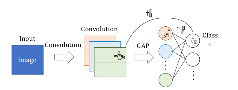
Convolutional Autoencoder (CAE) is a type of Deep Learning that combines an Autoencoder and a Convolutional Neural Network (CNN) for feature extraction of data [9]. In this study, CAE models were built using flame images taken by a High-speed camera during normal operation. CAE data analysis was then performed on all measured data, and an attempt was made to differentiate abnormal conditions by evaluating the differences between input and output images. The cases with small combustion oscillation levels (from Pos1 to Pos3) were used as training data for the detection of abnormal conditions.
The methods for evaluating the combustion instability using CAE are shown in Figure 4 and Eq. 1 - 3 below.
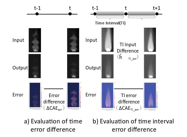
Here, 𝑛 is the number of pixels in the image, 𝛼 is the number of samples in the time interval before 𝑡, 𝛽 is the number of samples in the time interval after 𝑡, and 𝑥 is the luminance (normalization:0-1).
In the first method, as shown on the left of Figure 4 a) and in Eq.1, the time variation value (ΔCAEerr) of the residual sum of squares between the luminance of the input image (𝑥in) and luminance after CAE analysis (𝑥out) is defined as the Combustion Instability Index. In the second method, where focus was placed on the time interval corresponding to the sequential control of air flow as shown on the right of Figure 4 b) and in Eq.2, the amount of change between each interval (ΔCAETI_err) was defined as the Combustion Instability Index. In the results and discussion in Chapter 4, we confirm the validity of the evaluation index proposed in this study by comparing it with the Combustion Instability Index calculated by the conventional evaluation method (ΔImTI_err) as shown in Eq. 3, which does not use CAE.
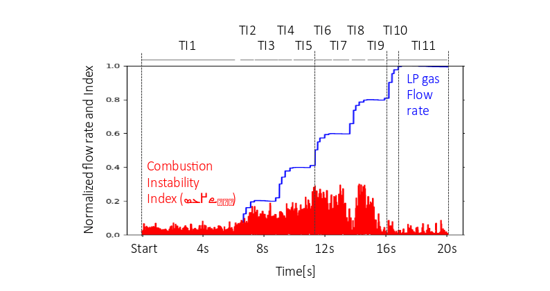
This study investigated the relationship between the Combustion Instability Index calculated from the flame image data analysis described above and the level of pressure fluctuation. In this study, combustion experiments were conducted with sequential control of air flow rate, and it was considered that the Combustion Instability Index also changes in steps according to the change in air flow rate. The Combustion Instability Index (ΔCAEerr), as defined in Eq.1 and indicated by the red line in Figure5, had a tendency of changing significantly around time intervals from TI6 to TI8.
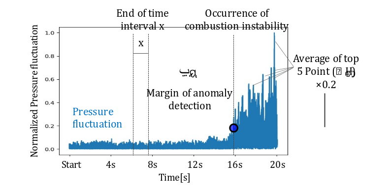
As shown in Figure6, the combustion oscillation level was evaluated as the average of the five maximum values of the pressure fluctuation level (p’N) in each case. The pressure fluctuation level was evaluated by the absolute value of amplitude. By evaluating the correlation between the Combustion Instability Index and the pressure fluctuation level for each section, we discussed in Chapter 4 whether the information obtained from the flame image could detect signs of increased pressure fluctuation. The time difference between the time of occurrence of combustion instability and the end of the previous time interval was defined as the margin of abnormality detection (ta), which was used in Chapter 4 as an index to evaluate the margin to the point of occurrence of increased combustion oscillation.
3.2. Grad-CAM
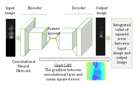
In this study, the Grad-CAM method [10] was applied to visualize which parts of the image were affected by the model in the feature extraction process by CNN described in section 3.1. The heatmap output shows the areas that affected the output value (Sc) by multiplying the features (Axyk) output by the gradient (αck) obtained by back-propagation. The calculation equation is shown in Eq.4.

Here, 𝑘 is the output of convolutional layer, Axyk is the feature at the x, y position, 𝑧 is the number of pixels in feature map, ωck is the weight parameter connecting output and input, and Sc is the output at class 𝑐.
As shown in Figure 7, this study focused on the gradient between the output of the convolution layer of the encoder section and the residual sum of squares calculated by Eq.2, and attempted to visualize in a heat map the part that affected the data analysis results. The state change of Combustion Instability Index (ΔCAETI_err) is evaluated in the CAE data analysis, and in the evaluation using Grad-CAM described in this chapter, the amount of change in the average value between each interval, shown in Eq.5, was also incorporated as an evaluation method so that the state of change in the area that affected the data analysis can be evaluated using image distribution.

Here, 𝛼 is the number of samples in the time interval before 𝑡 and 𝛽 is the number of samples in the time interval after 𝑡.
4. Results and Discussion
Data analysis of all cases was performed using the CAE evaluation method described in Chapter 3. Figure 8 shows the relationship between the combustion instability index (eq.2) and combustion oscillation level for each Pos with varying flame position.
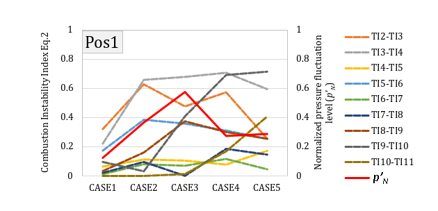
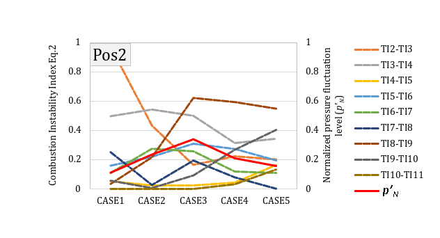
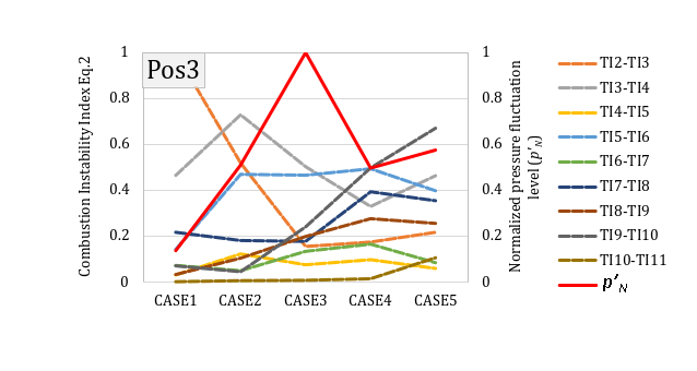
Figure 8. Relationship between Combustion Instability Index and pressure fluctuation level (p’N) in all test cases
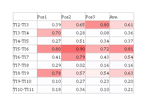
The combustion oscillation level was maximum at Pos3. This is considered to be closely related to the antinode of the acoustic mode formed inside the combustor. The combustion oscillation level was the largest in case 3 for all test data from Pos1 to Pos3. It is considered that there is a singularity in the fuel-air ratio which the combustion oscillation level increases. The correlation coefficient between the combustion instability index (eq.2) and the combustion oscillation level (p’N) was analysed (Table 2), and it was found that the interval used to calculate the combustion instability index, TI5-TI6, had the largest correlation coefficient. There is a possibility that a characteristic change in flame shape that leads to an increase in the combustion oscillation level has occurred in TI5-TI6.
Then, we organised the relationship between the pressure fluctuation level and the combustion instability index calculated from flame images in time interval from TI5 to TI6. Figure 9.1 plots the average of the pressure fluctuation level of the top five points against the luminance change of the High-speed camera image, calculated using the conventional index ΔImTI_err as shown in Eq. 3. Figure 9.2 plots the average of the pressure fluctuation level of the top five points against the Combustion Instability Index (ΔCAETI_err) calculated using Eq.2 proposed in this study.
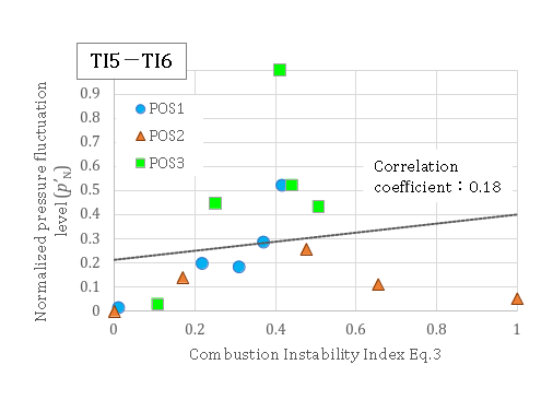
Figure 9.1. Relationship between Combustion Instability Index and pressure fluctuation level
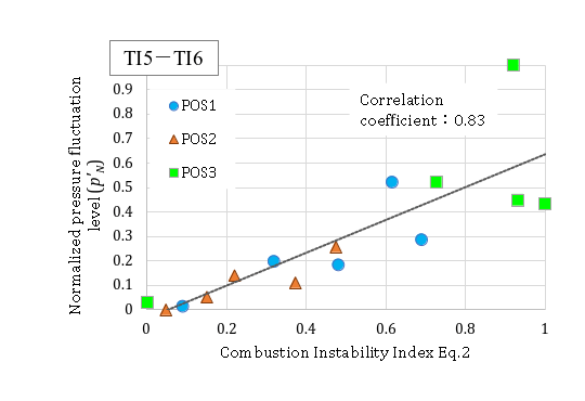
Figure 9.2. Relationship between Combustion Instability Index and pressure fluctuation level
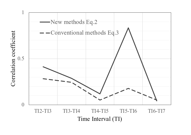
The proposed Combustion Instability Index has a correlation coefficient of 0.83 (in figure9.2), which indicates that it can detect the onset of combustion oscillation level better than the conventional method (in figure9.1). Figure 10 shows the results of correlation analysis between the Combustion Instability Index (ΔCAETI_err) and the combustion oscillation level for all data. The method proposed in this study had the tendency of showing higher correlations compared to the conventional method in all time intervals.
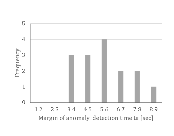
Then, in accordance with the definition shown in Figure 6, the relationship between the data obtained for time interval from TI5 to TI6 and the oscillation increase start time was analysed in order to quantitatively evaluate how many seconds before the start of oscillation increase can the signs of oscillation increase be detected. The results of the data analysis for all data (Figure 11) showed that the most frequent value of the detection time was from 5 to 6 seconds. Based on the above results, the Combustion Instability Index (ΔCAETI_err) proposed in this study is an effective evaluation index that can detect signs of increased oscillation in advance.
Next, we analysed the data using Grad-CAM as described in section 3.2 in an attempt to identify the elements in the image that had a significant impact on the Combustion Instability Index. In this data analysis, the evaluation index shown in Eq. 5 was used. As in the evaluation of the Combustion Instability Index, we focused on the amount of change in the interval mean in the Grad-CAM.
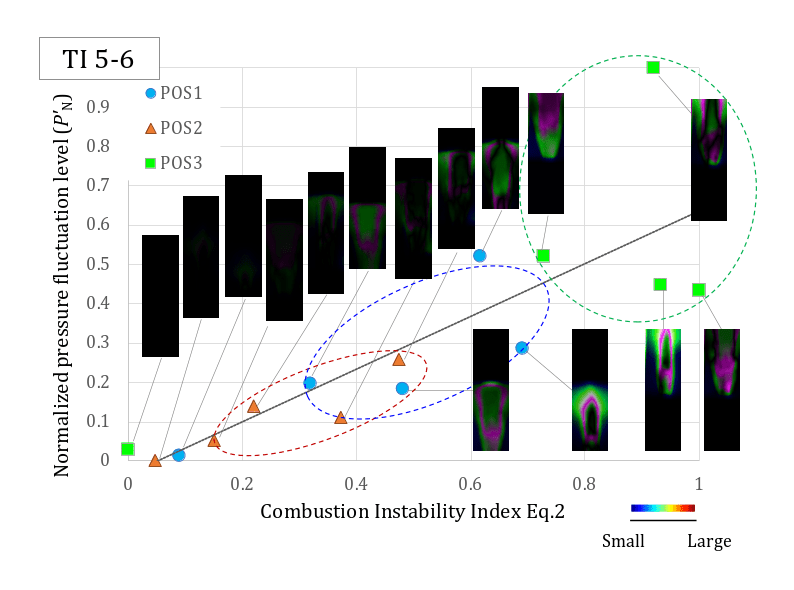
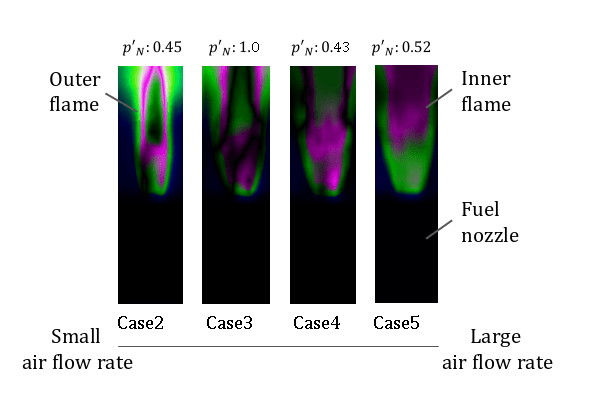
In the Grad-CAM image shown on the Figure 12, the inner flame near the nozzle outlet and the outer flame at the edge of the flame tended to be coloured red. Focusing on the flame position of Pos3 shown on the Figure 13, the red area shifts from the outer flame to the inner flame as the air flow rate is increased in the order of Case 2 to 5. Since the combustion oscillation level (P’N) reaches its maximum in Case 3 at the middle air flow rate, there is a possibility that there is a singularity where the coupling between combustion flame and acoustic mode is promoted and the oscillation increases during the transition process of air flow rate change. Qualitatively, the Combustion Instability Index increases as the combustion oscillation level increases in the order of Pos2, Pos1, and Pos3, as shown in the coloured circle in the Figure 13, suggesting that the evaluation index for combustion instability proposed in this study is effective.
5. Conclusion
In this study, in order to understand combustion instability phenomena in a simple way, the pressure fluctuation level and combustion flame images in various operations were measured using a simple combustion device consisting of a burner with a nozzle with a swirler and a rectangular cylinder with a visualization window. We focused on the flame images taken with a High-speed camera, used the Combustion Instability Index (ΔCAETI_err) calculated from Convolution Autoencoder (CAE) analysis, and discussed its relationship with the combustion oscillation level. At the same time, we applied the Grad-CAM data analysis method to visualize which part of the image is highly weighted in the feature extraction process for the Convolutional Neural Network (CNN) used in the calculation process of the Combustion Instability Index (ΔCAETI_err). The correlation between the Combustion Instability Index (ΔCAETI_err) proposed in this study and the combustion oscillation level was as high as 0.83, indicating the possibility of detecting the increasing trend of combustion oscillation level in advance. The results of the Grad-CAM data analysis, which allows visualization of the influence on the Combustion Instability Index (ΔCAETI_err), confirmed a tendency for the influence rate to shift from the outer flame to the inner flame with increasing air flow rate. Although there is a singular point where the combustion oscillation level increases with a specific air flow rate, qualitatively, the evaluation index for combustion instability proposed in this study was confirmed to be useful.
References
[1] McCartney M., Indlekofer T., and Polojke W., "Online Detection of Combustion Instabilities Using Supervised Machine Learning," in Proceeding of ASME Turbo Expo 2020, Turbomachinery Technical Conference and Exposition GT2020 September 21- 25.
[2] Lieuwen T., "Online Combustor Stability Margin Assessment Using Dynamic Pressure Data," Journal of Engineering for Gas Turbines and Power, Vol.127 No127 (2005) 478-482. View Article
[3] Gotoda H., Nikimoto H., Miyano T. and Tachibana S., "Dynamic Properties of Combustion Instability in a Lean Premixed Gas-Turbine Combustor," Chaos: An Interdisciplinary Journal of Nonlinear Science, Chaos 21, 013124(2011) View Article
[4] Peng J., Cao Z., Tu X., Yang S., Yu Y., Ren H., Ma Y., Zhang S., Chen S. and Zhao Y., "Analysis of Combustion Instability of Hydrogen Fueled Scramjet Combustor on High-Speed OH-PLIF Measurements and Dynamic Mode Decomposition," International Journal of Hydrogen Energy, Volume 45, Issue 23, 28 April 2020, Pages 13108-13118. View Article
[5] Lee S.-Y., Seo S., Broda J.C., Pal S. and Santoro R.J., "An Experimental Estimation of Mean Reaction Rate and Flame Structure during Combustion Instability in a Lean Premixed Gas Turbine Combustor," in Proceeding of the Combustion Institute, Volume 28, Issue 1, 2000, Pages 775-782 View Article
[6] Roncancio R., Gamal A. E. and Gore J. P., "Turbulent Flame Image Classification using Convolutional Neural Network," Energy and AI, Volume 10, November 2022, 100193 View Article
[7] Ramanan V. and Chakravarthy S. R., "Early Detection of Combustion Instability from Hi-speed Flame Images via Deep Learning and Symbolic Time Series Analysis," in Proceedings of Annual Conference of the PHM Society 2015, Vol./ No.1(2015)
[8] Zhou Y., Zhang C., Han X. and Lin Y., "Monitoring Combustion Instabilities of Stratified Swirl Flames by Feature Extractions of Time-Averaged Flame Images using Deep Learning Method," Aerospace Science and Technology,Volume 109, February 2021, 106443 View Article
[9] Guo X., Liu X., Zhu E. and Yin J., "Deep Clustering with Convolutional Autoencoders" International Conference on Neural Information Processing 2017, Neural Information Processing pp 373-382 View Article
[10] Selvaraju R. R., Cogswell M., Das A., Vedantam R., Parikh D. and Batra, D., "Grad-CAM: Visual Explanations from Deep Networks via Gradient-Based Localization" in Proceedings of the IEEE International Conference on Computer Vision (ICCV), 2017, pp. 618-626 View Article