Journal of Fluid Flow, Heat and Mass Transfer (JFFHMT)

ISSN: 2368-6111

Flashing Phenomena in Multiphase VOF Investigation for Water Purification

Tarek H Nigim

Mechanical Engineering, University of Alberta
Edmonton, AB, T6G 1H9, Canada
nigim@ualberta.ca

Abstract - This study explores the phenomenon of flashing within dedicated chambers, pivotal for water purification in multistage flash (MSF) systems. Introducing a new classification encompassing ideal, infinite, and finite flashing processes, we employ a computational approach using a two-phase Volume-of-Fluid (VOF) model. Our model accurately reproduces phase-change phenomena, free surface dynamics, and thermofluid behaviour. Validation against real-world data from operational flashing chambers precedes an examination of the effects of finite and infinite flashing processes on flow patterns and thermal performance. Our findings emphasize the significant influence of flashing process types, finite or infinite, on thermofluid behaviour within the evaporation zone. This study provides valuable insights into the complex multiphase dynamics of flashing, essential for optimizing MSF Desalination.

Keywords: multiphase; VOF; finite and infinite flashing; thermofluid behaviour; MSF, Water purification.

© Copyright 2024 Authors - This is an Open Access article published under the Creative Commons Attribution License terms Creative Commons Attribution License terms. Unrestricted use, distribution, and reproduction in any medium are permitted, provided the original work is properly cited.

Date Received: 2023-03-10
Date Revised: 2024-05-16
Date Accepted: 2024-05-28
Date Published: 2024-06-14

1. Introduction

The multistage flash (MSF) desalination encompasses an intricate system, with the flashing chamber emerging as a pivotal component facilitating diverse phases and fluid interactions [1]. Within this chamber, the exchange of energy and mass at its boundaries holds utmost importance for operational efficacy, alongside the consideration of non-equilibrium temperature difference (NETD = T_outlet – T_vapour) [2]. Here, an evaporation zone manifests, extending to the brine's free surface, where surface evaporation occurs through self-boiling [3] mechanisms triggered by pressure reduction, inducing a phase change phenomenon.

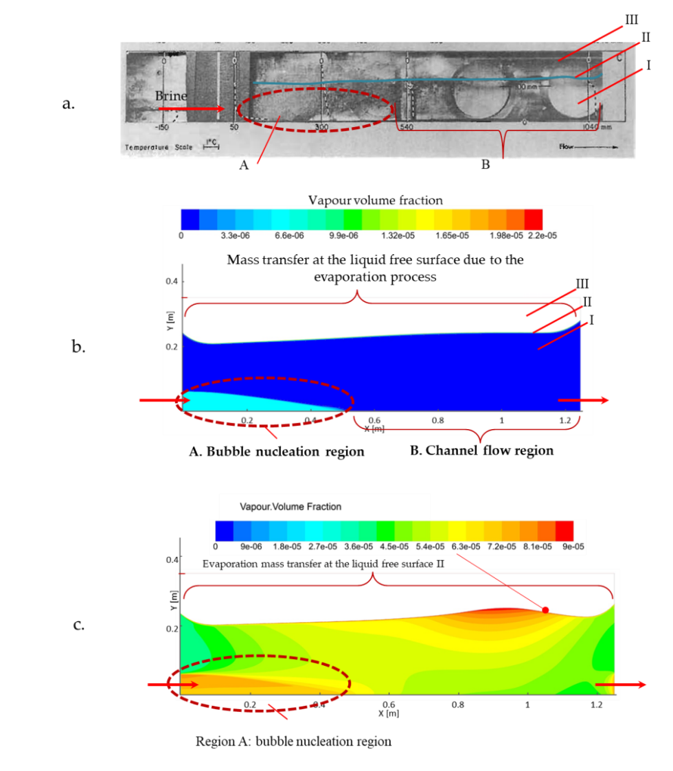
The flashing chamber can be divided into distinct layers and regions, as noted by Lior [4]. There are three vertical layers: I, which is the layer of brine flow near the base; II, the free surface or brine-vapour interface layer; and III, the vapour layer at the top. Additionally, two horizontal regions are identified: A, comprising the bubble nucleation region near the inlet with a submerged jet and recirculating flow; and B, representing the downstream channel flow, primarily unidirectional.

The flashing process within these chambers classifies into three types: ideal, finite, and infinite [5]. The flow dynamics within the evaporation zone are renowned for their complexity, featuring multiphase, turbulent, and unsteady characteristics, intertwined with diverse flow patterns and interactions [6].

This study focuses on analysing a simplified two-dimensional flow within a flashing chamber without baffles. Comprehensive understanding of flashing process, including the non-equilibrium temperature difference, is pivotal for optimizing the efficiency of the MSF desalination. Our principal objective is to employ a multiphase VOF model to anticipate thermofluid behaviour within the flashing chamber for both finite and infinite flashing flows.

2. CFD Model Description

Our computational approach relies on the FLUENT 14.5 two-phase VOF formulation [7, 8] to replicate the flashing process within an MSF desalination flashing chamber. This model incorporates two distinct phase-change mechanisms to delineate phase-change regions and determine the free surface shape. It is specifically tailored to simulate steady multiphase flow within a baffle-free flashing chamber. Due to computational constraints and the complexity of interpreting transient analyses, the model operates within a steady-state, two-dimensional framework.

Comparing our simulation results with available empirical data validates the model's accuracy in capturing the key phase-change mechanisms induced by the flashing process. Notably, vapor bubble formation is prominent at the chamber's inlet, gradually diminishing along its length. Furthermore, significant phase change and mass transfer occur at the liquid's free surface.

2.1. Volume of Fluid (VOF) Multiphase Model

To simulate two-fluid flow dynamics accurately, it is essential to consider factors such as density ratios, temperature jumps across the interface, surface tension effects, topological connectivity, and boundary conditions. Applications involving air-water dynamics, breaking surface waves, solidification melt dynamics, and combustion and reacting flows typically require a two-fluid flow simulation method.

The VOF method, available in the multiphase options of the FLUENT software, is a well-established and validated [9 - 15] approach for tracking interfaces between two or more immiscible fluids in free surface flows. The technique utilizes a group of rectangular cells near the interface to assign appropriate properties and variables to each control volume within the domain based on the local value of the liquid and vapour phase fractions.

The VOF model [7, 8] uses a single set of momentum, energy, and turbulent transport equations for all fluids and computes the volume fraction of each fluid in each computational cell throughout the domain to identify any emerging interfaces. However, it provides information only about the shared properties of the single-fluid mixture, which is its main limitation compared to a Eulerian model that solves individual momentum and continuity equations for each phase.

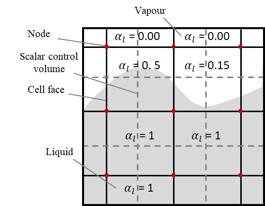
Figure 1 depicts a cluster of rectangular cells neighbouring an interface, with the liquid region shown in shaded form. In a flashing simulation, the liquid phase fraction is symbolized by α_l, while the vapour phase is represented by α_v in each cell within the computational domain. Three categories of cells can be identified: empty cells (where α_v), cells that are filled with vapour phase (α_v = 1), and cells that contain the interface between vapour and liquid phase (0 ˂ α_v ≤ 1). Suitable properties and variables will be assigned to each control volume within the domain, based on the local value of α_v α_v=1and α_l.

2.2. Phase Change Models

Both local thermal effects (saturation temperature) and mechanical effects (vapour pressure) are taken into account in our computational model for predicting flashing flow. Bubble formation and collapse are simulated using an indicator condition based on these mechanisms.

The Lee Wen Ho [17] model is used as a mechanistic model for phase change, representing the transition from liquid to vapour phase and vice versa. Vapourisation-condensation is determined by checking the temperature of the liquid phase (T_l). Mass transfer of the molecules occurs at the liquid-vapour interface, and kinetic energy is a function of the saturation temperature (T_sat) of the liquid. The local saturation temperature corresponding to the local pressure of the system is considered as an indicator.

If T_l ˃ T_sat (vapourisation), then

(1)

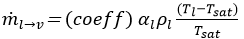
If T_v ≤ T_sat (condensation), then

(2)

where, = mass transfer rate from liquid to vapour phase, = mass transfer rate from vapour phase to liquid. =vapour phase fraction, =density of vapour [kg/m3], = density of liquid [kg/m3].

The coefficient, coeff, needs to be adjusted carefully to obtain the most accurate representation of performance. It is also referred to as a relaxation. To facilitate preliminary calculations when the diameter of the vapour bubbles is unknown, we set the value of coeff to 0.1, eliminating the need to define the diameter.

The mechanical effect is captured by an indicator based on a model proposed by Zwart et al [18] and derived from the generalized Rayleigh-Plesset equation. The indicator assumes that all bubbles in the system are of the same size, and vapour bubbles nucleate and grow when the local pressure of the phase is lower than the local saturation pressure. Conversely, vapour bubbles collapse and disappear when the local pressure (p) of the phase is greater than the local saturation pressure (pv). The indicator condition is developed based on these principles.

If p ≤ pv , then

(3)

(4)

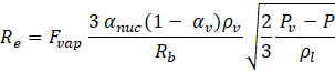
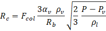
where, R_e= mass transfer source term connected to the growth of the vapour bubbles, R_c = mass transfer source term connected to the collapse of the vapour bubbles. R, 𝐹_𝑣𝑎𝑝= vaporization coefficient = 50, 𝛼_𝑛𝑢𝑐 = nucleation site volume fraction = 5*10-4, 𝑅𝑏 = bubble radius = 10-6 m, 𝐹_𝑐𝑜𝑙 = collapse coefficient = 0.01.

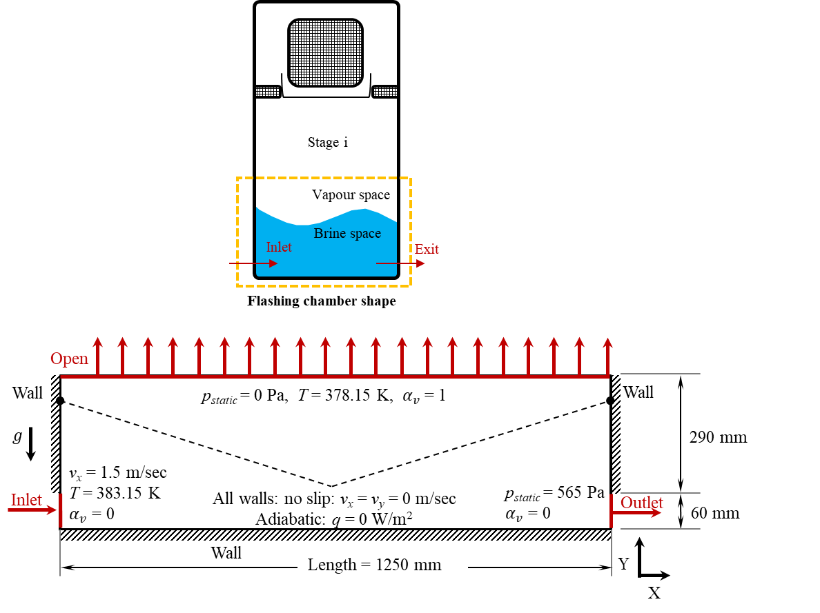
3. Computational Case Setup and Validation

In this study, we develop a computational model to simulate the evaporation zone in the first flashing chamber of a MSF desalination plant, validating its accuracy against data from the Sidi Krir plant in Alexandria, Egypt. The computational domain's dimensions (Figure 2) and operating conditions are sourced from published literature [19, 20]. The domain encompasses the chamber's geometry, bounded by walls on three sides, with a single inlet and outlet for the brine. Mesh generation results in 201,358 elements, including six inflation layers near the walls to enhance accuracy in resolving near-wall flows (Figure 2). The mesh refinement extends into the viscous sublayer near solid surfaces [7].

The model employs wall functions and the k – ε turbulence model. It is based on a 2D, steady-state, adiabatic, turbulent, and two-phase flow of liquid water and water vapor, without accounting for surface roughness. A pressure-based solution algorithm is used to derive the pressure, while the PISO algorithm resolves the pressure-velocity coupling. The study utilizes a collocated scheme, storing all variables, including velocity and pressure, at cell centres. To enhance precision, second-order upwind differencing is applied to the convective terms in the momentum, volume fraction, turbulence variables, and energy equations. Fluid properties are estimated from published sources [21, 22], with vapor pressure being a function of the local temperature. The simulation's accuracy is verified by comparing the model's results with measured values from the Sidi Krir plant.

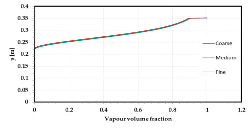
3.1. Mesh Resolution

In the analysis of multiphase flow featuring phase change and free surface prediction, accurate results necessitate the meticulous selection of mesh size. It is critical to employ a mesh size that is small, gradual, and lacking sudden changes in cell size to prevent the omission of phase change zones and achieve flow field resolution. The initial application of a coarse mesh aimed to establish mesh independence, as per the recommendation of [19, 20]. A range of meshes with quadrilateral rectangular shape elements, encompassing coarse (1.6 x 1.6 mm), medium (1.4 x 1.4 mm), and fine (1.2 x 1.2 mm) meshes, were subsequently evaluated using the current model and identical boundary and initial conditions as presented in (Figure 2) The pertinent variables, temperature, velocity magnitude, and vapour volume fraction, were extracted by traversing the flashing chamber at x = 0.6 m, randomly as shown in (Figure 3). Comparison of the predicted results showed that the maximum differences were insignificant, with temperature distribution, velocity distribution, and vapour volume fraction distribution being less than 0.03°C, 0.05 m/s, and 0.00625, respectively. These findings suggest mesh independence. To ensure precision, the outlet average temperature was compared for all three mesh sizes. The fine mesh size (378.7 K) exhibited the highest accuracy compared to the given outlet temperature of 379 K [19, 20]. Consequently, the fine mesh size was applied in all subsequent study cases. 

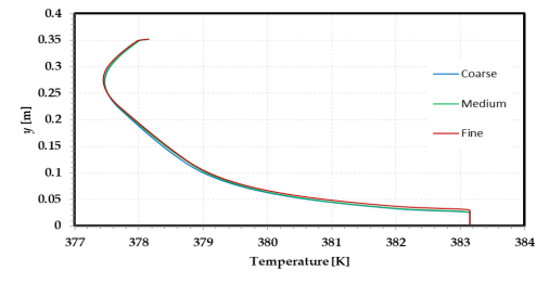
x = 0.6 m

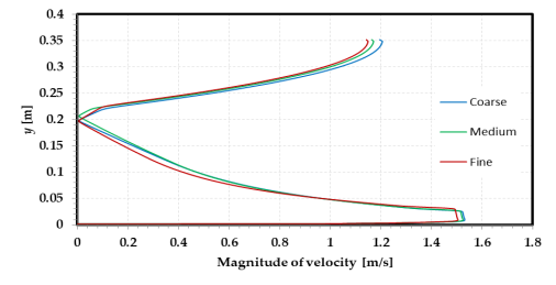
x = 0.6 m

x = 0.6 m

3.2. Validation

A significant challenge in predicting the behaviour of the flashing chamber lies in obtaining sufficient data to build and validate a computational model. Specifically, gathering detailed information about the interior of the chamber, such as bubble nucleation rate, bubble formation, recirculation zone size and length, brine level, and orifice shapes and numbers, is difficult. Additionally, the limited available data often lack specifics about measurement locations, methods, and uncertainties.

To address these challenges, our validation process included three main components:

A. Visualization of the Flashing Process & Phase Change Regions: Our simulation visualizes the formation and movement of vapor bubbles within the flashing chamber. This visualization helps in understanding the spatial distribution of the phase change regions and the dynamics of bubble formation and growth.

B. Evaluation of Operating Data: We validated our simulation by comparing it against available real plant data. Specifically, we compared the average temperature at the stage exit and the average vapor temperature above the liquid free surface. This comparison, presented in Table 1, shows good agreement with the actual plant values, indicating that our model accurately predicts the temperature distribution and phase change within the chamber.

C. Assessment of the Underlying Physics & Design Factors: The VOF multiphase model, well-established and validated in predicting liquid-gas interfaces and free surface shapes across various applications [9-15], was employed alongside the mechanistic Lee Wen Ho vaporization-condensation model [17] for vapor volume fraction prediction. Additionally, we independently validated the implementation of the Zwart et al vaporization-condensation model [18] within the Fluent VOF code using data from extensive experiments on isothermal flashing water flow in a converging-diverging nozzle by Abuaf et al [23]. The validation showed a strong correlation between our predicted values and the experimental data, reinforcing the accuracy of our model.

Furthermore, our simulation of the flashing process aligns well with the mechanism described in the introduction. Figure 4 illustrates that vapor bubbles form at the entrance of the flashing chamber and their generation decreases along the chamber's length. The simulation also accurately captures the phase change and mass transfer occurring at the liquid's free surface, the two primary mechanisms of phase change resulting from the flashing process. Regarding the brine level, the simulation predicts a level of 0.2 meters above the inlet, consistent with the design recommendations proposed by El-Dessouky et al [24], which suggest that the brine pool should be 0.2 meters higher than the gate height.

Table 1. Comparison of predicted results and measured values.

	Measured	Predicted	Relative Error [%]
Average outlet temperature[K]	379	378.6	0.1
Average vapour temperature[K]	375	377.7	0.7

4. Results

The developed model demonstrated the ability to accurately predict the free surface level and shape, as well as visualize the flashing process and phase change regions throughout the prediction field, regardless of whether it occurs under finite or infinite flashing flow conditions (Figure 4).

Figure 5 shows the flow fields observed in both finite and infinite flashing scenarios. These fields are characterized by the velocity magnitude and vector map with fixed length vectors, which are measured across the flashing chamber. Due to low tangential shear stress, the velocity magnitude near the free surface is significantly low. Additionally, the mixture comprises a higher proportion of vapour than the liquid phase above and away from the free surface, resulting in an increase in fluid speed due to the mixture density effect.

As shown in (Figure 5), the fluid movement is relatively high in the bubble nucleation region, which subsequently decreases along the channel flow region. However, at the brine exit, the fluid accelerates to the maximum due to area reduction.

The thermal performance of both finite and infinite flashing flows is shown in (Figure 6). The rate of flashing is directly linked to the thermal performance, or brine temperature field. The flashing process reduces the brine temperature, as demonstrated by the overall temperature field and the horizontal temperature traverses displayed in (Figure 6) The temperature decrease occurs in both the horizontal (x-) and vertical (y-) directions, but in different rates.

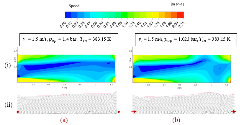
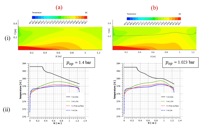
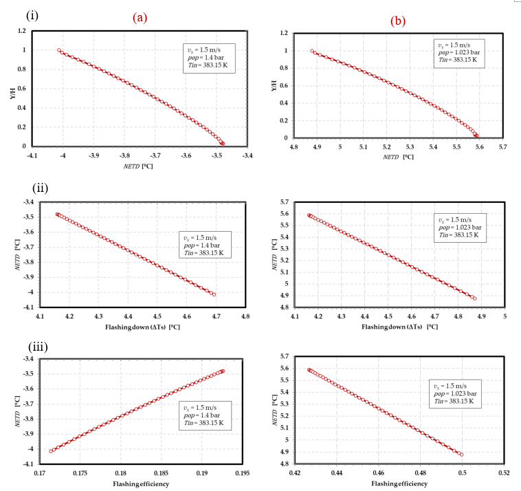
Figure 7 depicts the distribution of non-equilibrium losses (NETD) across the flashing chamber outlet orifice for both finite and infinite flashing scenarios. In Figure 7a, the NETD is shown to vary with depth, exhibiting a nearly linear decrease for finite flashing and a linear increase for infinite flashing. Specifically, for finite flashing (Figure 7ai), the NETD decreases from -4.01 to -3.48°C with increasing depth of the brine, while for infinite flashing (Figure 7aii), the NETD increases from 4.8 to 5.59°C. The relationship between NETD and flashing down (T_in-T_out) is presented in Figure 7b, where it is observed to be directly proportional for both scenarios. For finite flashing (Figure 7bi), the flashing down ranges from 4.16 to 4.69°C, while for infinite flashing (Figure 7bii), it ranges from 4.17 to 4.88°C. In Figure 7c, the relationship between NETD and thermal flashing efficiency (Flashing down/Flashing range) is depicted. For both finite and infinite flashing, a decrease in NETD corresponds to an increase in flashing efficiency. Specifically, the thermal flashing efficiency ranges from 0.171 to 0.192 for finite flashing (Figure 7ci) and from 0.425 to 0.5 for infinite flashing (Figure 7cii).

5. Discussion

This study examines particle paths and velocity distribution in both finite and infinite flashing conditions. In infinite flashing, the minimum velocity at the free surface maintains mass conservation, while a maximum speed of 1.88 m/s at the chamber's end upholds the conservation of energy. In finite flashing, the maximum speed is 1.9 m/s, also confirming energy conservation. The recirculation zone aids in bubble transport to the free surface, shedding light on the relationship between fluid flow and thermal behaviour, including turbulent kinetic energy conversion for vertical heat flow prediction.

The inlet velocity profile is a critical fluid dynamic parameter influencing the flashing process. Careful consideration of the inlet velocity profile is necessary for inter-stages and the final flashing chamber. An analysis showed that a uniform inlet velocity profile results in the closest average outlet temperature compared to available plant data, with tests conducted using three different unidirectional flow cases with varying inlet profiles [25].

The thermal performance of the flashing process varies between finite and infinite conditions. In infinite flashing, the temperature reduction due to phase change influences mass transfer and vapour distribution. Vertical temperature gradients dominate due to turbulent shear mixing, favouring vertical heat transfer. Positive NETD (Figure 7) is observed as the exit brine temperature exceeds the saturation temperature corresponding to the operating pressure. In finite flashing, the brine temperature decreases until reaching saturation temperature, after which no further phase change occurs. The exit brine temperature is lower than the saturation temperature, resulting in a negative NETD as shown in (Figure 7).

In our investigation of the flashing phenomena within the MSF desalination, an integral aspect of our analysis revolves around the NETD. The NETD serves as a critical parameter in assessing the efficiency and performance of the flashing chamber, providing insights into the thermal losses inherent in the system. In this discussion, we delve into the implications of the NETD values obtained for both finite and infinite flashing scenarios, exploring the factors influencing these values and their significance in optimizing the MSF.

In the context of finite flashing, it is ideal for the NETD to approach zero, as stated in prior literature [5]. However, our predicted results indicate an average calculated value of -3.74°C for the NETD. This discrepancy suggests a thermal loss within the flashing chamber, signifying the need for additional energy input to facilitate subsequent flashing processes.

Conversely, for infinite flashing, the average calculated value of the NETD is 3.8°C. While this may appear slightly higher than typical operational values [25] observed in existing plants, it falls within the expected range for flashing chambers without baffles.

Several factors contribute to these observations. Firstly, the simulated flashing chamber represents the initial stage within the MSF system, thereby experiencing the highest thermal losses. Moreover, the absence of a baffle within the simulated chamber, coupled with insufficient time for complete flashing to occur, exacerbates thermal losses. Additionally, the limited length of the flashing chamber impedes the attainment of thermal equilibrium conditions, further contributing to elevated thermal losses. Addressing these factors may involve optimizing the design of the flashing chamber, potentially incorporating baffles to enhance efficiency and allow for more complete flashing. Moreover, extending the length of the chamber could facilitate closer approximation to thermal equilibrium conditions, thereby mitigating thermal losses and improving overall system performance.

Overall, the thermofluid performance of the flashing process is a complex phenomenon that is affected by various factors such as the temperature gradient, mass transfer rate, and vapour volume fraction distribution. Understanding the differences in thermal performance between finite and infinite flashing conditions is crucial in designing and optimizing the flashing process to achieve higher efficiency and reduce energy consumption.

Within the domain of CFD, we must underscore the significance of subtle result variations. For instance, a mere 0.1% difference in validation outcomes, as observed using the VOF model, can have substantial real-world ramifications. In industries with stringent performance standards, even a one-degree temperature change can lead to significant energy losses and reduced system efficiency, underscoring the need for precision in CFD simulations, especially in multiphase contexts.

6. Summary and Conclusion

A numerical method was developed to predict the multiphase flow field during flashing flow using a FLUENT VOF code implementation. The model considered thermal and mechanical effects for phase change during the flashing process and was tested with three different mesh sizes to ensure accuracy. The model was evaluated for MSF desalination systems and found to match real plant values. Infinite and finite flashing were classified, and their effects on the flashing chamber performance were analysed based on operational parameters. The simulation results provided insights into heat transfer, mass transfer, and fluid dynamics during the flashing flow evaporation process. Design factors such as non-equilibrium temperature difference, flashing down, and flashing efficiency were estimated.

Optimizing flashing chamber performance requires achieving a NETD value of zero, indicating that the flashing process concludes precisely at the chamber exit. Achieving this ideal scenario may necessitate adjustments such as extending the chamber length or adjusting the flow rate. However, both infinite and finite flashing are associated with thermal losses to the system, requiring careful consideration. While the NETD is a crucial indicator of flashing chamber performance, additional metrics such as flashing rate and bubble nucleation frequency are necessary for a comprehensive evaluation.

The computational method can assist in the design and optimization of MSF systems by identifying ideal operating conditions and system parameters. Overall, this study provides valuable information for the design and optimization of MSF desalination systems through computational modelling.

Acknowledgements

This work was funded through a postgraduate Research Fellowship from the College of Engineering and Informatics, University of Galway, IRELAND.

References

[1] A.H. Khan, "Desalination Processes and Multi-Stage Flash Distillation Practice," Elsevier, Amsterdam, 1986.
[2] R. Rautenbach, S. Schäfer, and S. Schleiden, "Improved equations for the calculation of non-equilibrium temperature loss in MSF," Desalination, vol. 108, pp. 325-333, 1996. View Article
[3] T. H. Nigim and J. A. Eaton, "CFD prediction of flashing processes in a MSF desalination chamber," Desalination, vol. 420, pp. 258-272, 2017. View Article
[4] N. Lior, "Some basic observations on heat transfer and evaporation in the horizontal flash evaporator," Desalination, vol. 33, pp. 269-286, 1980. View Article
[5] T. H. Nigim, "Novel classification of multistage flash desalination via finite and infinite flashing: Investigating thermofluid dynamics under varying inlet flow rates employing validated multiphase CFD simulations," Computers & Chemical Engineering, vol. 179, 2023. View Article
[6] O. Miyatake, T. Fujii, T. Tanaka, and T. Nakaoka, "Flash evaporation phenomena of pool water," Heat Transfer Jpn. Res., vol. 1, pp. 393-398, 1975. View Article
[7] ANSYS Fluent Theory Guide, Release 14.5, 2016.
[8] J. H. Ferziger and M. Peric, "Computational Methods for Fluid Dynamics," Springer, New York, 2002. View Article
[9] W.F. Noh and P. Woodward, "SLIC (Simple Line Interface Calculation)," in Proceedings, Fifth International Conference on Fluid Dynamics, A.I. van de Vooren and P.J. Zandbergen, Eds., Lecture Notes in Physics 59, Berlin, Springer, 1976, pp. 330-340. View Article
[10] B.D. Nichols and C.W. Hirt, "Numerical simulation of boiling water reactor vent-clearing hydrodynamics," Nuclear Science and Engineering, vol. 73, pp. 196-209, 1980. View Article
[11] C.W. Hirt and B.D. Nichols, "Volume of fluid (VOF) method for the dynamics of free boundaries," Journal of Computational Physics, vol. 39, pp. 201-225, 1981. View Article
[12] S. Kvicinsky, F. Longatte, J.L. Kueny, and F. Avellan, "Free surface flows: experimental validation of volume of fluid (VOF) method in the plane wall case," in Proceedings of the 3rd ASME, JSME Joint Fluids Engineering Conference, San Francisco, California, 1999.
[13] R. Saurel and R.A. Abrall, "Multiphase Godunov method for compressible multifluid and multiphase flows," Journal of Computational Physics, vol. 150, pp. 425-467, 1999. View Article
[14] D.M. Hargreaves, H.P. Morvan, and N.G. Wright, "Validation of the volume of fluid method for free surface calculation: the broad-crested weir," Engineering Applications of Computational Fluid Mechanics, vol. 1, pp. 136-146, 2007. View Article
[15] V. Hernandez-Perez, "Gas-Liquid Two-Phase Flow in Inclined Pipes," Ph.D. thesis, University of Nottingham, 2008. View Article
[16] T.H. Nigim and J.A. Eaton, "Simulation of the flashing processes in a MSF desalination stage," in Desalination for the Environment: clean Water and Energy, EDS, Rome, Italy, May 2016. View Article
[17] W.H. Lee, "A Pressure Iteration Scheme for Two-phase Modeling," Technical Report LA-UR 79-975, Los Alamos Scientific Laboratory, Los Alamos, New Mexico, 1979.
[18] P.J. Zwart, A.G. Gerber, and T.A. Belamri, "Two-phase flow model for predicting cavitation dynamics," in Fifth International Conference on Multiphase Flow, Yokohama, Japan, 2004.
[19] K.M. Mansour and H.E.S. Fath, "Numerical simulation of flashing process in MSF flash chamber," Desalination and Water Treatment, vol. 51, pp. 2231-2243, 2013. View Article
[20] K.M. Mansour, H.E.S. Fath, and O. El-Samni, "Computational fluid dynamics study of MSF flash chambers sub-components; I - vapor flow through demister," in The Fifteenth International Water Technology Conference, IWTC15, Alexandria, Egypt, 2011.
[21] N.B. Vargaftik, B.N. Volkov, and L.D. Voljak, "International tables of the surface tension of water," Journal of Physical and Chemical Reference Data, vol. 12, pp. 817-820, 1983. View Article
[22] M.H. Sharqawy, J.H. Lienhard V, and S.M. Zubair, "Thermophysical properties of seawater : a review of existing correlations and data," Desalination and Water Treatment, vol. 16, pp. 354-380, 2010. View Article
[23] N. Abuaf, B.J.C. Wu, G.A. Zimmer, and P. Saha, "A Study of Non-Equilibrium Flashing Of Water in a Converging-Diverging Nozzle: Volume 1 - Experimental," United States Nuclear Regulatory Commission Office of Nuclear Regulatory Research, 1981.
[24] H.T. El-Dessouky and H.M. Ettouney, "Fundamentals of Salt Water Desalination," Elsevier Science B.V., Amsterdam, the Netherlands, 2002.
[25] T. H. Nigim, "Computational Modelling of Thermofluid Flashing in MSF Desalination," Ph.D. Dissertation, University Galway, 2017.