Journal of Fluid Flow, Heat and Mass Transfer (JFFHMT)

ISSN: 2368-6111

Optimization of Powertrain Parameters of a Battery Electric Vehicle for Shuttle Service Usage

Murat Otkur¹, Abdullah Khalfan¹

¹College of Engineering and Technology
American University of the Middle East, Kuwait
murat.otkur@aum.edu.kw, 57966@aum.edu.kw

Abstract - Although Electric Vehicles (EVs) had been used for transportation since the end of 19th century, they were superseded by Internal Combustion Engine (ICE) propelled vehicles due to limited performance and low driving range problems. In the last 2 decades considering the performance advancements and price drop in the battery technology, EVs started to gain significant attention and usage. Furthermore, they have zero in use emissions, reducing the effects of fossil fuels in terms of air pollution and Global Warming (GW). However, compared to ICE propelled vehicles main drawbacks like low driving range and long charging durations limit the favourability of EVs. Considering special use cases such as shuttle services in specified areas, these drawbacks lose their importance. The proposed study involves, the selection design and optimization of an EV to be used in the American University of the Middle East (AUM) campus considering the main objective as to complete the daily tasks with a single charge during the night. A longitudinal vehicle model is generated for the EVs in MATLAB/Simulink, a benchmarking vehicle is selected using vehicle model outputs and parameter optimization for battery capacity and final drive ratio (FDR) is performed. The final design has 32.47 % less battery capacity, 1.94 % less vehicle weight and 7.901 seconds 0 – 25 kph vehicle acceleration duration, 17.86 % less than the original selected configuration. The results of this study will serve as a valuable input for the autonomous driving car development project planned at AUM.

Keywords: Battery Electric Vehicle, Longitudinal Vehicle Modelling, Parameter Optimization, MATLAB/Simulink

© Copyright 2023 Authors - This is an Open Access article published under the Creative Commons Attribution License terms Creative Commons Attribution License terms. Unrestricted use, distribution, and reproduction in any medium are permitted, provided the original work is properly cited.

Date Received: 2023-08-20
Date Revised: 2023-09-26
Date Accepted: 2023-10-04
Date Published: 2023-10-16

1. Introduction

First EV was invented at the end of the 19th century in 1884 by Thomas Parker [1] and it was using lead-acid batteries which had been introduced to the market about 25 years prior. Due to properties of this type of batteries, EVs had significant disadvantages such as low driving range and long charging duration considering the level of technology at the end of the 19^th century. Internal Combustion Engine (ICE) propelled vehicles superseded the EVs at the beginning of the 20th century because they offered longer driving range, easy refuelling, low fuel cost and they were more accessible to consumers. Later, an energy crisis occurred between 1970 and 1980 and led to insufficient energy reserves for industrial processes and domestic uses making EVs come back to market [1]. At the beginning of the new millennium, EVs had gained considerable usage ratios despite their drawbacks and expensive prices compared to conventional vehicles. Furthermore, considering special use cases such as shuttle services in specified areas, these drawbacks of EVs lose their significance where driving range and charging durations are not the main concerns. This is because these shuttle services are not required to cover long distances and they have ample time to charge the batteries overnight.

ICE propelled vehicles are powered by fossil fuels, particularly, petroleum to derive their long range effect. Unfortunately, fossil fuel combustion is a major cause for Global Warming (GW) due to the high carbon dioxide (CO₂) content, classified as greenhouse gas (GHG) emissions, in the exhaust gases. EVs are applied in many instances to eliminate the fossil fuel consumption, increase vehicle efficiency and to reduce carbon emissions [2], [3]. Furthermore, EVs are uniquely fitted with regenerative braking which enables to recover and convert the braking kinetic energy into electrical energy that is stored in the battery of the vehicle which increases the overall efficiency and improves driving range. However, a major drawback that EV technology faces is the inaccurate modelling of the vehicle system and its operations under varying conditions [3].

Another major factor that has led to the increased adoption of EVs is the reduction in prices of energy storage solutions. Miri et al. developed a model to depict this price decrease from $500 per kWh in 2012 to $160 per kWh by the year 2025 [4]. Despite all these pros and cons, drivers have yet to widely adopt the use of EVs for their day-to-day use. This is mainly because of the limitation in the availability of infrastructure for charging stations to recharge the small-capacity batteries. This is coupled with the long durations required for charging. Solutions to these issues are being developed rapidly with the depletion of energy reserves looming. As a result of the advancements in battery and electric motor technologies, EV development has made significant progress in the recent decades.

Simulations are important in the engineering design process to test a system before implementation while reducing production cost and time [5]. A trade-off between the vehicle range and battery cost should be established because they are inversely proportional. This trade-off is achieved using optimization to determine the optimum solution for the use case. Simulations are also very valuable for optimization algorithms. MATLAB/Simulink has been widely used to evaluate aspects of EV design such as the battery power flow which is the distribution of electrical power from the battery to the vehicle. Sri Kaloko et al. investigated the flow of electricity form the battery to the vehicle’s energy system in MATLAB/Simulink [6]. To derive a mathematical model of an EV, physical equations were determined and used to represent each component in the EV drive train. Similarly, Mohd et al. analysed the power flow specifically during motoring manoeuvre where batteries are charged via regenerative braking [2]. Another example is performed by Srujana et al. where MATLAB/Simulink was utilized to develop a model for the battery electric vehicle and analyse it [7]. The work endeavours to use the same tool to develop a model for an EV to assess its operation and observe its functioning. The battery’s State of Charge (SOC) estimation is of vital importance for providing intelligence to the driver about the remaining range for EVs. Within this perspective Bhatt et al. developed an EV model with the capability of SOC estimation taking into consideration different operating conditions and temperature profile of the batteries using MATLAB/Simulink software [8].

There are different optimization algorithms utilized to find optimal solutions of mathematical models. Generally, optimization algorithms use single or multiple objective functions alongside constraints that limit the mathematical model of a system according to its real-life operation. In [9], the genetic algorithm (GA) method was used to optimize the battery capacity and the final drive ratio (FDR) for New European Driving Cycle (NEDC) profile. Optimization can also be used to reduce the energy consumption of an EV for instance suggesting optimizing the speed profile [2].

2. Methodology

Despite the drawbacks of EVs like low range and high charging duration, considering specific usages such as operation in a limited area, EVs can be considered as the optimum solution. Within this study powertrain optimization of an EV that will be used in the AUM campus as a shuttle service car was performed. The shuttle service cars in AUM operates 14 hours a day between 8:00 AM and 10:00 PM. Currently, they are used in 2 shifts as morning and afternoon and charged 2 times as during the night and daytime between the shifts.

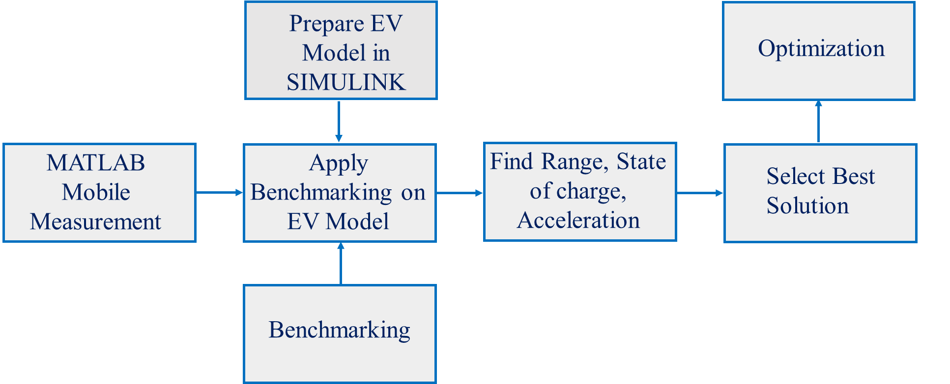
The aim of this study is to define the optimum parameters for an EV that is charged overnight, start its duty with full SOC in the morning and complete all the driving cycle profiles with a single charge. Within this perspective first, the driving cycle (DC) of the shuttle cars was determined using MATLAB mobile software for both shifts. Afterwards a mathematic longitudinal vehicle model for EVs was generated in MATLAB/Simulink considering 2 scenarios: Performing daily tasks via following the generated DC and 0 to maximum allowed vehicle speed in campus (25 kph) acceleration. The model was used to assess 5 commercial EVs including the one used in the AUM campus. Via comparison of the final SOC and acceleration duration, the most suitable EV for usage in AUM campus was determined. The study continued with the optimization of the EV parameters as battery capacity and FDR using the particle swarm optimization (PSO) method in MATLAB. The methodology flowchart is depicted in Figure 1.

2.1. Determining the Driving Cycle

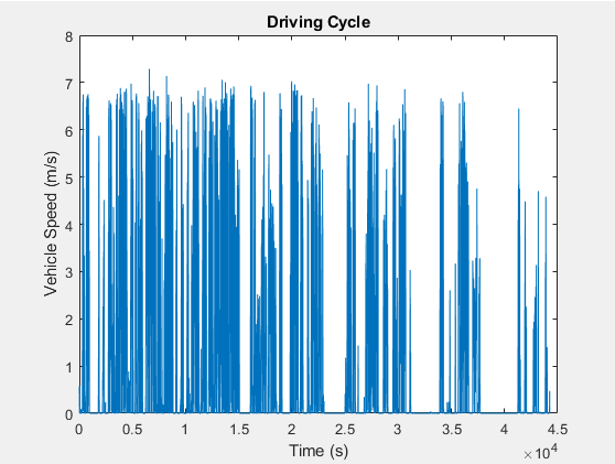
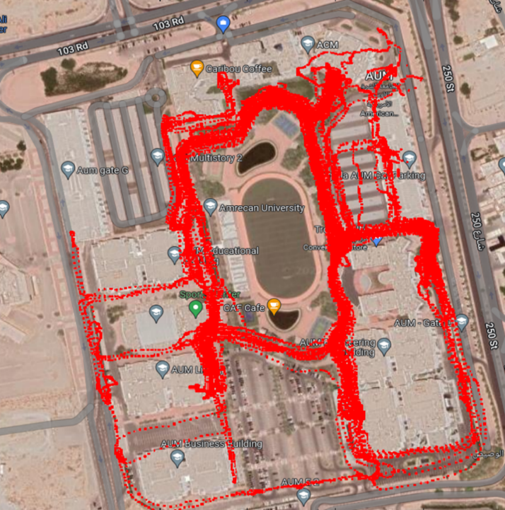
Vehicle driving tests and vehicle driving propagations aid and sustain the cycle configuration, allowing the determination of whether the arrangement is practical for the intended use. Driving cycles (DCs) are a second-by-second schedule of timestamp-referenced speed values for the replica car to achieve. A DC is necessary to lessen the number of time-consuming and resource-draining on-road tests, as well as to reduce test durations and effort. The relationship between vehicle speed and elapsed time is the primary focus of a DC. Within this perspective, MATLAB Mobile software is used to collect vehicle speed second-by-second data. A mobile device mounted on the EV shuttle service car is utilized for taking the measurements which started approximately at 8:00AM and finished at 10:00PM. Measured DC vehicle speed and X, Y coordinate position in AUM campus are shown in Figures 2 and 3 respectively.

2.2. Development of the Longitudinal Dynamics EV Model

The developed EV model consists of 3 main parts: calculation of the road load, determination of the tractive effort on the wheels and SOC prediction.

Road Load Calculation

The road load consists of 3 components: Aerodynamic resistance, rolling resistance, and grade resistance.

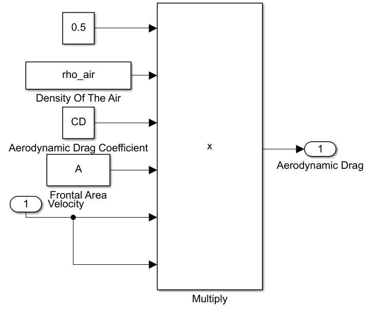
Aerodynamic resistance is the force that opposes an object's motion through a fluid or gas medium. The term aerodynamic or air resistance is used when the fluid is a gas, such as air. According to the shape of the vehicle, the aerodynamic resistance coefficient is calculated experimentally. The calculation of the aerodynamic drag resistance force is represented below.

(1)

where:

• ρ_air = density of the air (1.225 kg/m³ at sea level and 15 ᵒC)
• CD = aerodynamic drag coefficient
• A = frontal area
• v = velocity of air

The Simulink subsystem for calculating the aerodynamic load is shown in Figure 4, where the input is vehicle speed with the unit m/s.

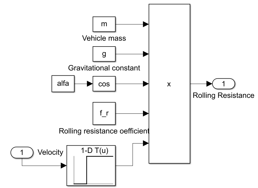
Rolling resistance is the energy that a vehicle must transfer to the tires to keep moving across a surface at a constant speed. The phenomenon known as hysteresis is the primary cause of rolling resistance. The energy lost as the tire rolls across its footprint is referred to as hysteresis. The vehicle's engine must work harder to compensate for the energy loss. The formula is written as:

(2)

where:

• m = vehicle mass
• g = gravitational constant
• 𝛼 = inclination angle
• f_r = rolling resistance coefficient

The Simulink subsystem for calculating the rolling resistance is shown in Figure 5. Where the input is vehicle speed in the unit m/s. The vehicle speed input is utilized to zero rolling resistance at negative and zero vehicle speed values as equation 5 results with rolling resistance values even for stationary conditions.

Grade resistance is the gravitational force acting on the EV on an inclined road, and can be calculated with the following formula:

(3)

where:

• m = Vehicle Mass
• g = Gravitational Constant
• 𝛼 = Inclination Angle

The Simulink subsystem for calculating the grade resistance is shown in Figure 6.

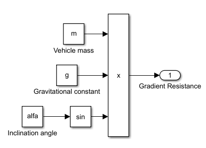
Considering the levelness of the AUM campus, the gravitation road load is negligible and assumed to be zero in this study.

Tractive Force Calculation

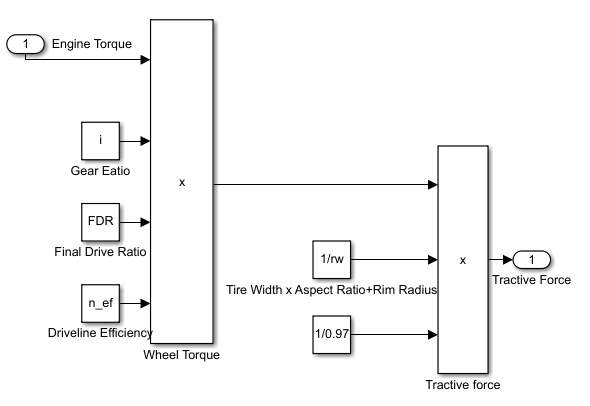
In EVs used for Golf Carts, the electric motor is placed in the rear axle. The wheel torque is calculated using the formula below:

(4)

where:

• T_w = Wheel torque
• T_e = Engine torque
• i = Gear ratio
• FDR = Final drive ratio
• 𝜂_ef = Driveline efficiency

Gear ratio is assumed to be 1 as a single speed transmission is used in the calculations. The tractive force at the wheels is determined using the formulas below where 0.97 coefficient is used to calculate the rolling wheel (r_w) radius due to the deformation of the tire under vehicle weight.

(5)

(6)

The Simulink subsystem for calculating the tractive force is shown in Figure 7 where the input is electric motor torque with unit Nm.

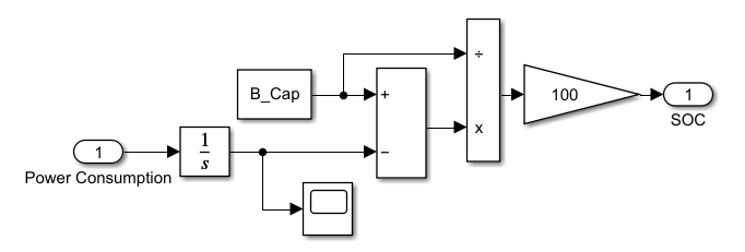
State of Charge (SOC) Calculation

EVs deplete their batteries considering acceleration and cruising maneuvers and charge their batteries during braking/deceleration instances. Furthermore, considering the energy conversion from the battery to the wheels an efficiency value needs to be used during battery depletion and it is defined as 98% within this study. Similarly, during regenerative braking an efficiency of %95 is used where kinetic energy is assumed to be converted to electrical energy in the battery. The SOC value was calculated using the following formula.

(7)

where:

• C_releasable = Releasable capacity
• C_rated = Battery rated capacity

The Simulink subsystem for SOC calculation is shown in Figure 8 where the input is instant power consumption value with the unit kW.

The vehicle parameters used in the longitudinal EV model are summarized in Table 1.

Table 1. Parameters used in longitudinal vehicle dynamics calculation.

Parameter	Value
Drag coefficient	0.5
Gear reduction	1
Final drive ratio	7
Air density	1.234 kg/m3
Frontal area	1.5 m2
Rolling resistance coefficient	0.2
Driveline efficiency	0.95
Inclination angle	0 °

Final MATLAB/Simulink EV Models

Two MATLAB/SIMULINK models were developed with the purposes of calculating the SOC during a DC following maneuver and 0 – 25 kph acceleration maneuver as shown in Figures 9 and 10 respectively. Both models were developed based on the equations described in sections 2.2.1 to 2.2.3.

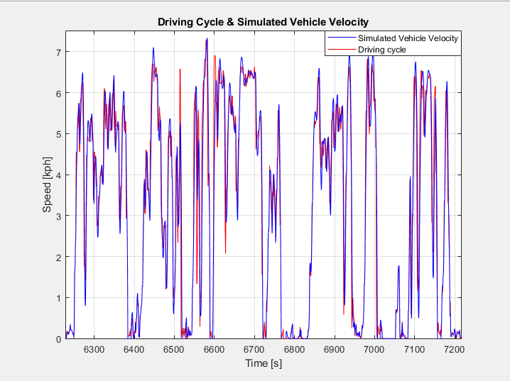
Considering the SOC calculation, a PID controller that manipulates the acceleration pedal position is tuned so that the vehicle longitudinal velocity follows the DC set speed second by second values as shown in Figure 11. The PID coefficients are provided in Table 2.

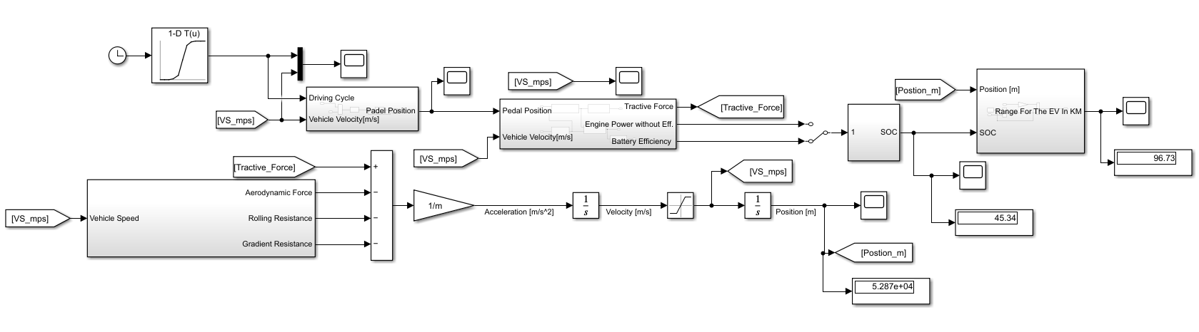
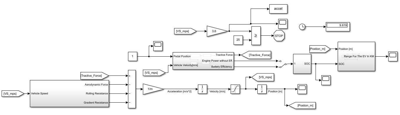
Table 2. PID controller gains.

Controller Gain	Proportional (P)	Integral (I)	Derivative (D)
Value	0.75	0.5	0.5

2.3. Alternative EVs Benchmarking

A benchmarking table comparing the powertrain parameters of 5 EVs including the golf cart used in the AUM campus is listed in Table 3. The essential design parameters used in the modeling and simulation of the Auto Power electric vehicle, which was selected from a benchmarking study of five distinct electric golf carts brands XHUNHU, LGAO, Zhongyi, Suzhou Eagle and Auto Power, are tabulated in the table. These parameters are then implemented in a MATLAB/Simulink equation-based analytical model in order to simulate vehicle performance.

2.4. Optimization of the Battery Capacity and FDR Parameters with PSO

Range of the EVs and their longitudinal acceleration performance depends on various powertrain parameters such as electric motor (EM) torque curve, FDR, tire radius and battery capacity. Upshifting the EM torque curve, increasing FDR, reducing tire radius will improve acceleration performance. Battery capacity is the main factor effecting vehicle range, however on the other hand degrades acceleration performance as it will increase the vehicle mass. Therefore, finding optimum parameters for determining the battery capacity and FDR is considered as an optimization problem. The population-based stochastic optimization method known as Particle Swarm Optimization (PSO) is widely used to solve multi-input multi-output (MIMO) system optimization problems. Within this study PSO algorithm is applied in order to determine the optimum parameters for the EV.

Considering EVs, having a higher battery capacity improves driving range. However, for the specific problem in this study the required range to complete daily tasks according to vehicle measurements is defined as 53.28 km. The optimization problem is defined in such a way that at the end of the day battery SOC should be 20 % in order to have 1.2 safety factor. PSO parameters used in MATLAB PSO optimization script are listed in Table 4.

Cost function used the PSO algorithm is defined based on having 20 % SOC at the end of the cycle and have minimum 0-25 kph acceleration.

(8)

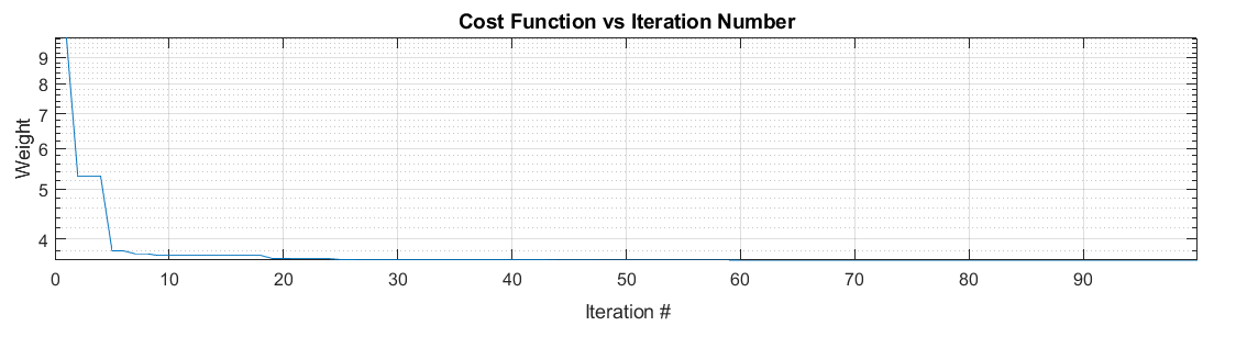
Acc is the 0-25 kph acceleration duration in seconds. In order to reduce the weight of the acceleration goal in the cost function a target of 6 secs is provided. Although the number of maximum iterations is set to 100, after 50th iteration (Figure 12), the final values are converged as 18.8032 and 3.8899 kWh for FDR and battery capacity respectively.

Table 3. Parameters of the 5 EV golf carts.

Car model	Dimensions	Weight	Tire Dia.	Battery	Motor	Max Torque	Rated Speed
Auto Power	3.92 x 1.198 x 1.83 m	605 kg	15 inches	48 V/ 120 Ah	48 V/ 4 kW	25.5 Nm	1500 rpm
Zhong Yi	4.47 x 1.21 x 1.98 m	655 kg	12 inches	48 V/ 140 Ah	48 V/ 5 kW	15.9 Nm	3000 rpm
Xunhu	3.82 x 1.2 x 1.9 m	700 kg	18 inches	48 V/ 170 Ah	48 V/ 3 kW	19.1 Nm	1500 rpm
Suzhou Eagle	4.37 x 1.18 x 1.89 m	640 kg	10 inches	48 V/ 250 Ah	48 V/ 5 kW	16 Nm	3000 rpm
LGAO	3.7 x 1.38 x 1.65 m	850 kg	12 inches	60 V/ 120 Ah	60 V/ 4 kW	17.74 Nm	3000 rpm

Table 4. PSO parameters.

Parameter	N# of var.	N# particles for init.	Upper boundaries	Lower boundaries	Max iteration number
Value	2	15	30, 6	4, 1	100

4. Results

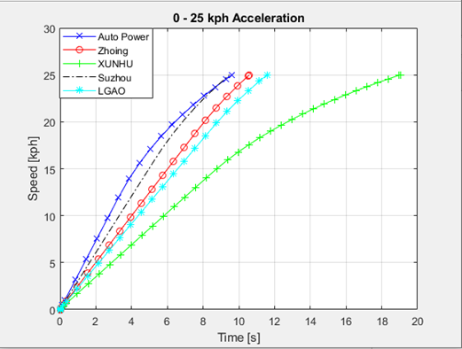
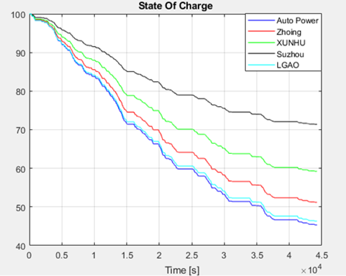
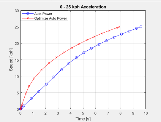
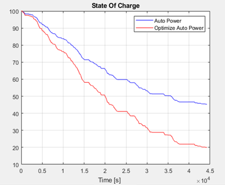
The 5 alternative EVs listed in section 2.3 were simulated for the driving cycle and acceleration maneuvers and the results are summarized in Table 5 and plotted in Figures 13 & 14. The best solution is determined as Auto Power golf cart with 45.34 % for SOC at the end of the DC and 0 – 25 kph acceleration in 9.619 s as the shortest duration. Having a larger battery capacity is preferable when it comes to EVs since it increases their range. However, for the sake of this analysis, a target range of 53.28 km is used based on the vehicle measurements. The optimization algorithm is set in such a way that at the end of the cycle a final battery SOC of 20% with safety factor value of 1.2 is achieved at the end of the day. The final values for battery capacity and FDR are calculated as 3.8899 kWh and 18.8032 respectively. Simulation results for the acceleration and DC following maneuvers are shown in Figures 15 & 16 respectively. As expected, a higher FDR resulted in better acceleration performance reducing the maximum speed of the vehicle. However, as there is speed limit in AUM campus as 25 kph, the top speed reduction does not have any negative impact at this study.

Table 5: Results of the 5 EV Golf Carts.

EV Model	Range (km)	SOC	0 – 25 kph in (s)
Auto Power	96.73	45.34	9.619
Zhong Yi	106.7	51.19	10.59
Xunhu	123.7	59.22	19.04
Suzhou Eagle	183.8	71.39	9.476
LGAO	96.45	46.31	11.58
Optimized Auto Power	66.58	19.9	7.901

5. Conclusion

Electric battery vehicles are superior alternatives to traditional fossil fuel-powered vehicles, especially when considering their impact on the environment and public health. While there may be some arguments against electric battery vehicles, such as their up-front costs or limited range compared to fossil fuel vehicles, these drawbacks can be mitigated through proper planning and infrastructure development. This project addressed a crucial topic as the EV has the potential to significantly reduce greenhouse gas emissions and improve air quality on campus. The EV powertrain designed aimed to have optimized performance and efficiency with minimized costs.

A benchmarking study was conducted of already available EV golf carts in the market with the brands: Auto Power, Zhong Yi, Xunhu, Suzhou Eagle, and LGAO. The best EV solution selected for the AUM campus shuttle service was Auto Power. The Auto Power EV powertrain parameters were optimized using MATLAB/Simulink software using PSO algorithm. Before optimization, the EV’s range, state of charge and 0 – 25 kph acceleration duration were 96.73 km, 45.34 and 9.619 s respectively. A significant drop was noted in all parameters after optimization process as the range (km), SOC and 0 – 25 kph acceleration were 66.58 km, 19.9, and 7.901 s respectively. The optimized powertrain can perform the daily tasks on a single charge and has much better acceleration performance.

It is recommended that the AUM adopt the proposed EV powertrain as the primary mode of transportation on campus. This will not only reduce the university's carbon footprint but also serve as a model for other institutions and communities looking to transition to more sustainable transportation options. Additionally, the results of this study will be used for the autonomous driving car development project to be developed in AUM.

References

[1] A. O. Kıyaklı and H. Solmaz, H, "Modeling of an Electric Vehicle with MATLAB/Simulink" in International Journal of Automotive Science and Technology, 2019, vol. 2, issue 4, pp. 9-15. View Article
[2] T. A. T., Mohd, M. K., Hassan and W. M. K. A. Aziz, "Mathematical modelling and simulation of an electric vehicle" in Journal of Mechanical Engineering and Sciences, 2015, vol. 8, pp. 1312-1321. View Article
[3] F. Adegbohun, A. Jouanne, B. Philips, E. Agamloh and A. Yokochi, "High Performance Electric Vehicle Powertrain Modeling, Simulation and Validation" in Energies, 2021, vol. 14, 1493. View Article
[4] I. Miri, A. Fotouhi and N. Ewin, N. "Electric vehicle energy consumption modelling and estimation-A case study" in International Journal of Energy Research, 2021, vol. 45, issue 1, pp. 501-520. View Article
[5] D. McDonald D, "Electric Vehicle Drive Simulation with MATLAB/Simulink" in Proceedings of the 2012 North-Central Section Conference, 2012, pp. 1-24.
[6] B. S. Kaloko, M. R. Soebagio and M. H. Purnomo, "Design and Development of Small Electric Vehicle using MATLAB/Simulink" in International Journal of Computer Applications, 2011 vol 24, issue 6, pp. 19-23. View Article
[7] A. Srujana, A. Srilatha and S. Suresh, "Electric Vehicle Battery Modelling and Simulation Using MATLAB-Simulink", 2021, vol. 12, issue 3, pp. 4604-4609. View Article
[8] A. Bhatt, "Planning and application of electric vehicle with MATLAB/Simulink" in IEEE International Conference on Power Electronics, Drives and Energy Systems, PEDES, 2016, pp. 1-6. View Article
[9] A. Dinc and M. Otkur, "Optimization of Electric Vehicle Battery Size and Reduction Ratio Using Genetic Algorithm" in Proceedings of ICMAE 2020 - 2020 11th International Conference on Mechanical and Aerospace Engineering, 2020, pp. 281-285. View Article