Journal of Fluid Flow, Heat and Mass Transfer (JFFHMT)
ISSN: 2368-6111

Volume 9 - Year 2022 - Pages 157-164
DOI: 10.11159/jffhmt.2022.019
Enhancement of an Experimental Methodology for the Investigation of Contact Heat Transfer at High Pressures
Tim Göttlich1, Thorsten Helmig1, Nicklas Gerhard2, Thomas Bergs2 and Reinhold Kneer1
1Institute of Heat and Mass Transfer, RWTH Aachen University
Augustinerbach 6, 52056 Aachen, Germany
goettlich@wsa.rwth-aachen.de; helmig@wsa.rwth-aachen.de; kneer@wsa.rwth-aachen.de
2Laboratory of Machine Tools and Production Engineering, RWTH Aachen University
Campus-Boulevard 30, Aachen, Germany
n.gerhard@wzl.rwth-aachen.de; t.bergs@wzl.rwth-aachen.de
Abstract - Besides the mechanical description of technical systems, a thermal modelling is frequently required. For technical systems consisting of several individual components, the contact heat transfer coefficient is an essential boundary condition between the individual components. This parameter is mainly influenced by the surface structure and roughness of the contact partners as well as the applied contact pressure. However, although the influencing parameters are well known, an analytical determination is quite difficult. Therefore, an experimental quantification is mandatory. So far, experiments in literature have primarily focused on the investigation of contact heat transfers at moderate loads up to 100 MPa. Nevertheless, there are some applications where solids are in contact at very high pressure and resulting heat transfer between them plays an essential role, such as the interface between the tool and the workpiece during machining. The aim of this work is to present an enhanced experimental methodology to determine contact heat transfers at high loads. In this approach, infrared thermography is used to measure the temperature data, which is consequently used to solve an inverse problem using the conjugate gradient method, which provides the corresponding contact heat transfer coefficients. Furthermore, first experimental results for a load-dependent heat transfer for loads between 200 and 1200 MPa are presented and occurring effects are discussed.
Keywords: Contact Heat Transfer, Inverse Heat Transfer, Infrared Thermography, High Pressure.
© Copyright 2022 Authors - This is an Open Access article published under the Creative Commons Attribution License terms Creative Commons Attribution License terms. Unrestricted use, distribution, and reproduction in any medium are permitted, provided the original work is properly cited.
Date Received: 2022-09-30
Date Accepted: 2022-10-12
Date Published: 2022-11-04
1. Introduction
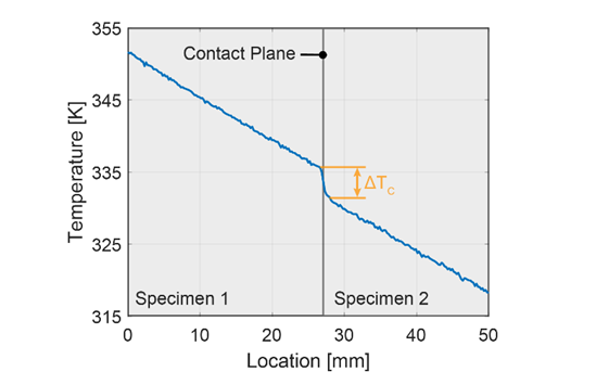
Due to the increasing demand for high manufacturing accuracy and quality, a precise thermo-mechanical description of the machine tool is mandatory. A sound knowledge of the temperature field is important in order to determine the temperature-related expansion of the various components. An important boundary condition for the thermal coupling of the temperature fields of the individual subcomponents is the contact heat transfer coefficient. This parameter is introduced as the real contact area AR is much smaller than the nominal geometric area AN due to the microscopic roughness of the technical surfaces. The actual contact area for metallic bodies is usually only 1-2 % of the nominal geometric area [1]. This leads to a restriction of the heat flux, resulting in a temperature drop across the contact plane, which can be seen exemplary in Figure 1. Using the heat flux ![]() which flows across the contact plane and the resulting temperature drop ΔTc, the contact heat transfer coefficient hc can be defined as follows:
which flows across the contact plane and the resulting temperature drop ΔTc, the contact heat transfer coefficient hc can be defined as follows:

Although the phenomenon has been studied since the 1930s and the main influencing variables are known, an analytical description is still very difficult.
Due to the complex interaction of surface geometry, elasto-plastic mechanical behavior and thermal modeling, open questions remain. Cooper [2] developed an analytical approach in the 1960s, which was later further developed by Mikic [3]. In this approach, the contact heat transfer is analyzed on the basis of the geometric description of the contact surfaces, the mechanical deformation of the contact surface caused by the contact pressure and the thermal behavior in the contact zone. In addition to these theoretical approaches, several experimental studies on contact heat transfer have also been conducted. In this context, the most common and simplest measurement method is the steady-state method. In this method, the surfaces of the specimens to be tested are compressed with a predefined force and then subjected to a steady-state heat flux. Several thermocouples are inserted into the specimens at uniform intervals to record the line-shaped temperature profile across the two specimens. The recorded temperature profiles are then extrapolated to the contact plane to determine the temperature drop occurring there. By means of the observed temperature drop ΔTc and the applied heat flux , the contact heat transfer can thus be quantified analogously to Equation 1. Using this experimental setup, Asif and Tariq [4] have determined heat transfer coefficients for different metal pairings. Sponagle and Groulx [5] have studied the impact of different interstitial media on contact heat transfer. While Liu et al [6] focused more on the influence of temperature in the contact plane on contact heat transfer. Although this experimental setup is widely used and numerous studies have been made, it has some shortcomings. First, it takes a long time to reach the required steady state, often several hours [7]. Second, the thermocouples must be inserted invasively into the samples, which can affect the temperature field in the specimen [8]. Burghold et al. [9] have therefore presented an alternative setup in which the temperature data of the specimens are determined using infrared thermography. The temperature detection is much more sensitive compared to thermocouples and temperature changes can be detected quickly. Using a transient evaluation method, time-dependent contact heat transfer coefficients can be estimated from the recorded temperature fields. This can be done, for example, using the conjugate gradient method developed by Alifanov [10] or the sequential function estimation procedure (SFEP) according to Beck et al. [11]. However, this is associated with a significantly higher computational effort, whereas the duration of the experiment is significantly shorter with this method. Although contact heat transfers have been studied for several decades, the focus of experimental research has been on contact heat transfers at moderate loads up to 100 MPa [12]. However, there are a few applications where solids come into contact with each other at much higher pressures, such as at the interface between the tool cutting edge and the workpiece during machining, where the contact pressures can reach several hundred MPa. For this purpose, there are numerical studies [13, 14] that show that the contact heat transfer reaches very high values of 100.000 or even 1.000.000 W/m²K, which is 1 or 2 orders of magnitude higher than the values experimentally studied so far. However, only individual operating points are investigated and not progressions over a larger pressure range. Furthermore, these results are based on numerical investigations and should be validated by experiments. Therefore, for a better understanding, fundamental experimental studies in a larger pressure range are necessary to better understand the phenomena that occur.
2. Experimental Setup
2. 1. Test Rig
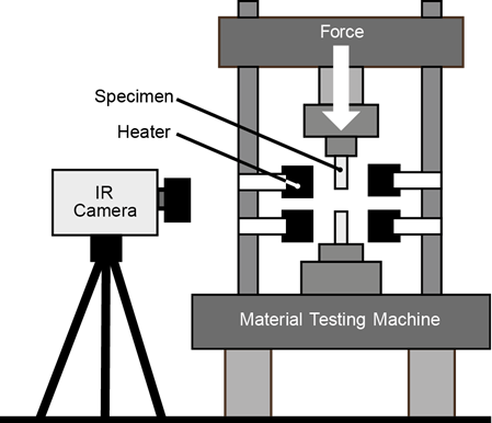
The experimental setup for the present investigations is the same as presented by Burghold et al. [9] and Helmig et al. [15], except that the specimen geometry is adjusted. A schematic of the experimental setup is shown in Figure 2. The main component consists of a servo-hydraulic material testing machine with a maximum test force of 100 kN, controlled by a PID controller. To measure the actual force, a strain gauge with a sampling frequency of 100 Hz is installed in the yoke of the press. The upper specimen is mounted on a vice which is fixed on the hydraulic cylinder, while the lower specimen is mounted on a vice which is fixed on the press table. Initially, the two specimens are heated by two independent heaters to reach the specified set temperatures. The heaters contact the side surfaces of the specimens as shown in Figure 2. Since the calibrated measurement range of the IR camera is from 30 °C to 125 °C, the upper sample is heated to a temperature between 110-120 °C, while the lower sample is tempered to 30-40 °C. The heating phase is monitored by thermocouples inserted in holes outside the IR visible surface. By the time the samples have reached the specified temperatures, the heating bars are pneumatically retracted and the upper sample is pressed onto the lower sample. While the specimens are pressed together, their temperature distributions on the front faces are recorded temporally and spatially using the infrared camera. The IR camera used is an Infratec ImageIR 5300, which can detect mid wavelength infrared in the range from 3.7 to 4.8 μm. The camera lens used for the investigations offers a pixel pitch of 30 μm at a working distance of 300 mm and a resolution of 320x256 pixels. Thus, the observed area is 9 x 7.68 mm, which can be used for subsequent analysis. This provides good spatial resolution and, with a recording frequency of 100 Hz, also good temporal resolution, which is necessary to provide good resolution of the transient local temperature changes.
2. 2. Specimen
Compared to Helmig et al [15], the specimen geometry was slightly changed in order to reduce the manufacturing effort. The specimens consist of a square with a base area of 20x20 mm and a height of 60 mm. As described in the previous section, the force of the test rig is limited to 100 kN. With a contact area of 20x20 mm = 400 mm², this results in a maximum contact pressure of 250 MPa.
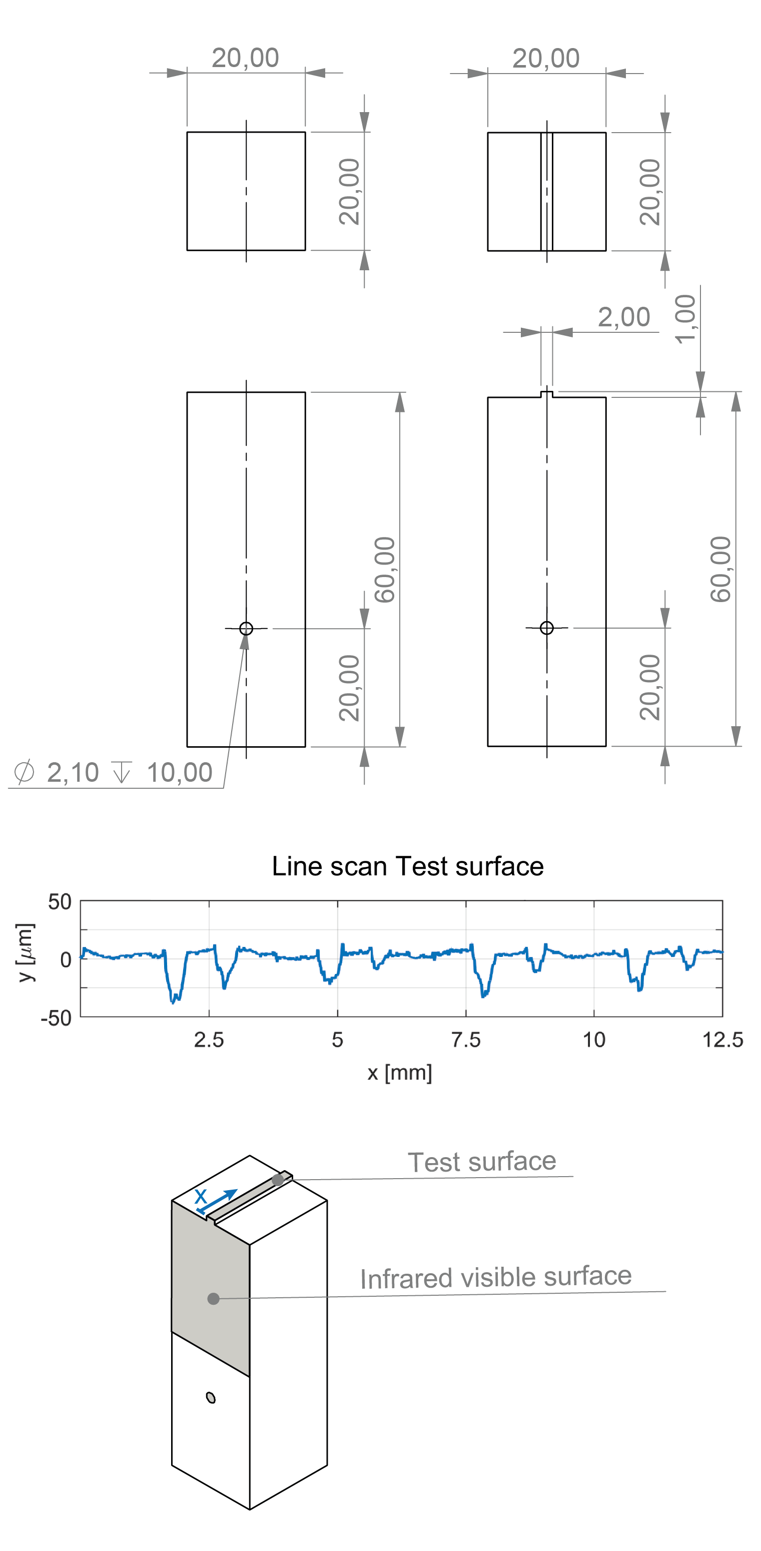
Since much higher pressures are to be investigated in the present work, the nominal contact area between the specimens must be reduced. Therefore, the new geometry of the upper and lower specimen differs in shape. As can be seen on the left side of Figure 3, the lower specimen has a flat surface. The upper specimen, on the other hand, has a 1 mm x 2 mm elevation in the center, which reduces the contact area between the two specimens to 40 mm² by a factor of 10. The visible surfaces of the specimens, on which the temperature field is recorded with the infrared camera, are grinded down to obtain as flat a surface as possible. This surface is finally coated with a thin layer of black paint with a known emissivity of about ε = 0.95 to minimize the influence of ambient radiation [8]. The test specimens are made of AISI 1045 steel, and the test surfaces are all milled with the same milling parameters using the rolling face of the milling cutter. The resulting surface roughness is Rq 8 mm and Rz 40 mm. To quantify and map the surfaces, line profiles will be recorded using a Mahr MarSurf10 surface profilometer. An example of surface measurements is shown in Figure 3. In each test repetition, specimens with the same surface parameters are pressed on top of each other at nine different pressures, evenly spaced between 200 and 1200 MPa. The tests are performed with three pairs of specimens and repeated three times per load point, gradually increasing the load.
3. Methodology
In the first step of the evaluation methodology, the specimen geometries in the IR images are mapped on a numeric grid using an edge algorithm. This searches for the largest temperature gradients and then marks the outlines of the sample geometry as it is significantly warmer than the ambience. In Figure 4a, the infrared image frame can be seen in the with the associated temperature field and isotherms. It is easy to see how the temperature profile propagates radially from the contact. In the second image, the resulting sample geometry is then marked in yellow, and the surrounding area can be seen in blue. In the next step, the contact plane with the corresponding contact points is defined, also by means of the edge algorithm. The contact points can be seen with a black line in image in Figure 4b. Based on the detected geometry and boundaries, a thermal simulation is created applying the two-dimensional heat conduction equation to determine the temperature Tsim(x,y,t,hc) shown in Equation 2, where the parameters ρ, cp and k are the thermophysical properties density, heat capacity and thermal conductivity, respectively.
These properties are assumed to be constant for the upper and lower specimens, which is justified due to the relatively small change in temperature. Since the heat conduction equation is a partial differential equation, its solution requires accurate boundary and start conditions. In the two-dimensional simulation three different boundary conditions are considered, which are visualized in image 3 of Figure 4. Ω1 represents the contact heat transfer coefficient as a boundary condition between the two specimens. Ω2 is an adiabatic boundary condition. Although an exchange via radiation between the bodies is to be expected, this can be neglected due to the low temperatures. The same is true for convective transport between the two specimens. Ω3 is the coupling boundary condition between the recorded region and the rest of the body. There, the values from the measurement for the respective time step are taken as boundary condition for the temperature. The resulting temperature field of the set up thermal simulation can be seen in Figure 4c. The algorithm for solving the inverse problem is based on the methodology of Alifanov [10] and Ozisik [16]. Here only a short version about the evaluation procedure is given, for a more detailed description the reader is recommended to refer to the given literature. The evaluation methodology is divided into three main steps. First, for a current iterative contact heat transfer coefficient hc, the resulting temperature field is calculated using the built simulation. Then, the parameter hc is systematically optimized by minimizing the difference between the measured temperature Tmeas and the simulated temperature Tsim. This is summarized by the criterion function J for each iteration step i, which can be seen in Equation 2.
This iterative process is repeated until the objective function reaches the previously defined termination criterion. Once the optimized simulation and the measurement have reached the highest possible agreement, indicated by the stagnation of criterion J, the iterative process is terminated and the obtained result is taken as the sought boundary condition.
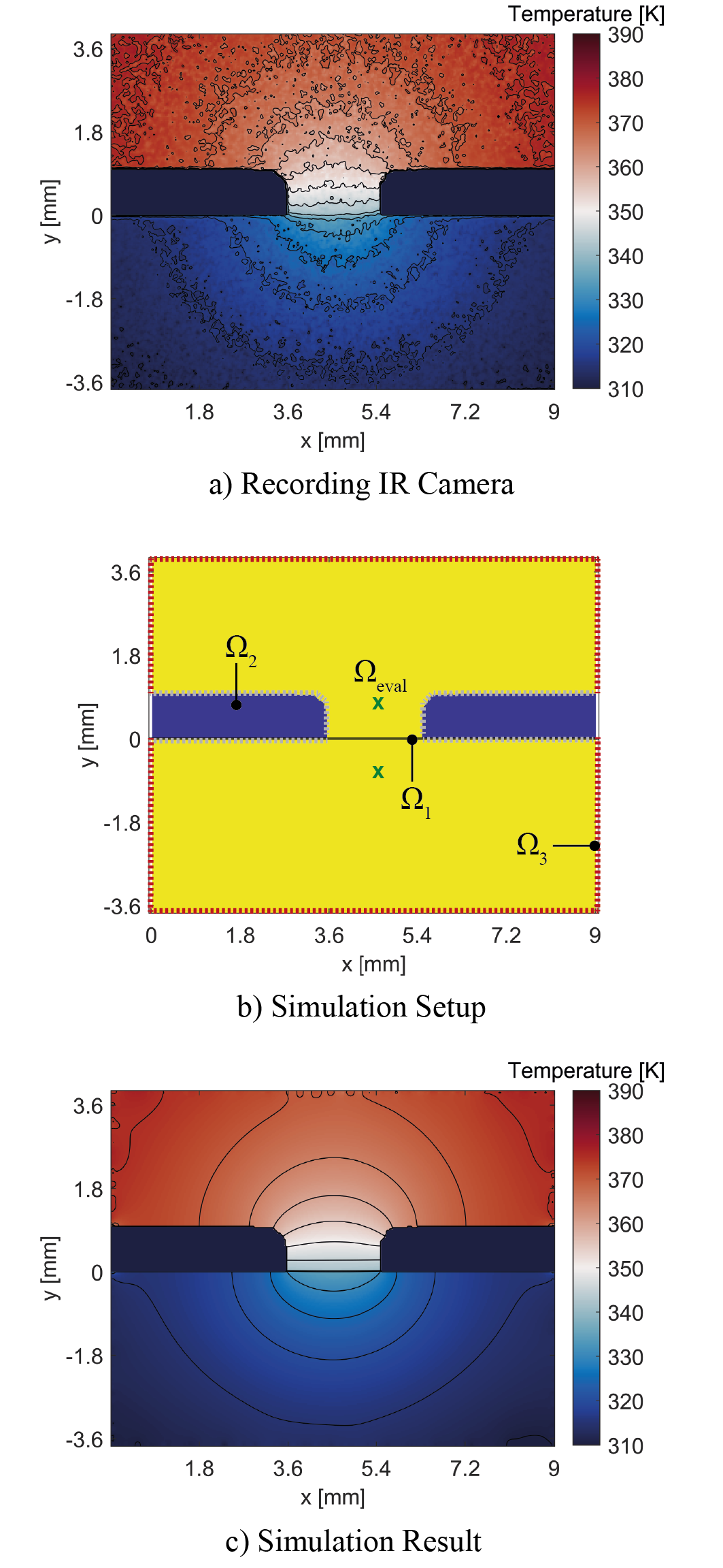
a) Recording of the temperature equalization process using the infrared camera
b) Data processing of IR recordings including determination of specimen geometry and contact edge
c) Setup and running of the simulation to solve the inverse problem to determine contact heat transfer coefficient.
4. Results
Figure 5 shows the calculated time-dependent contact heat transfer coefficient on the top as an example for specimen pair 1 at a contact pressure of 840 MPa. The diagram on the bottom shows the temperature profiles of the upper and lower specimen at the evaluation points marked by Ωeval and the green crosses in Figure 4b at a distance of 1 mm from the contact plane.
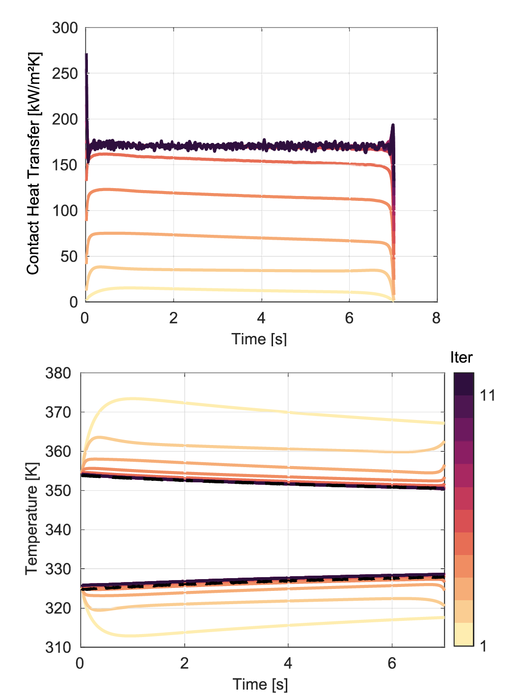
Bottom: Corresponding local temperature trends from experiment and inverse evaluation. The upper line shows the temperature trend of the upper specimen at the previously initiated evaluation point, while the lower lines correspond to the lower one. The evolution of the heat transfer coefficient over the course of the iterations is shown by the colored lines referring to the colorbar on the right side of the figure. The black dashed line shows the measured temperature trend.
In the first iteration step, the sought boundary condition is estimated to be 0 kW/m²K, therefore the temperature change is relatively small since no heat is transferred across the interface. The black dashed line shows the measured temperatures at the evaluation point. It can be seen how the simulated temperature profile gradually approaches this from the first iteration step. It is noticeable that the temperature profile from the final iteration step of the upper specimen coincides with the measured profile, while the lower one also matches the measured profile well, but a small deviation remains. The contact heat transfer coefficient in the top image shows well how it increases with the increasing number of iterations. The result of the last iteration shows a constant course over time at approx. 170 kW/m²K. This constant progression is to be expected due to the constant force imprint, since the contact heat transfer coefficient is proportional to the applied pressure according to Cooper [2]. Thus, this is a first indicator of the validity of the calculated result. The small deviations from a linear course are due to measurement uncertainties. The elevation after 7 seconds is due to the evaluation methodology. There, the individual results of the respective iteration steps are marked according to the color legend on the right side, so that the development can be observed over the iteration.
Figure 6 shows on the top the summarized results for the three specimen pairings for a contact pressure of 200 - 1200 MPa. Here, for each evaluation point, the transient contact heat profile shown in Figure 5 is averaged over the period of 2-4 seconds. Here, each measuring point was repeated three times per pressure. For a better examination of the data, a fourth-degree polynomial curve is fitted to the respective measuring points using the Matlab function "Bisquare". First of all, it is noticeable that the contact heat transfer coefficient for the specimen pairings present here with the corresponding test surfaces reach values of 50 - 540 kW/m²K. It can be clearly seen that the heat transfer increases with increasing contact pressure for all three pairs of specimens. However, in the pressure range 200-550 MPa, a logarithmic or flattening curve can be observed, whereas in the pressure range 550 - 1200 MPa, an exponential or steeply increasing curve can be observed. Figure 6 shows at the bottom the derivative of the course at the top with respect to the contact pressure. There, the previously described course is highlighted again in more detail, as the changes can be recognized better. It can be clearly seen how the slope decreases for both specimens up to the inflection point, marked by the black crosses, at a contact pressure of approx. 550 MPa. The three specimens also show the same gradient curve in the low load range, which is marked with Regime 1, only with a constant offset up to the inflection point. From then on, it can be seen how the slope increases progressively and clearly exceeds that of Regime 1. However, it can also be seen in the top figure that in the higher load range of Regime 2, the difference between the three specimen pairings decreases. It is noticeable that the three measurement repetitions per pressure point are very close to each other and consequently the standard deviation remains low, which is a good indicator of the stability and reproducibility of the evaluation method. However, the scatter between the individual measurement points increases with increasing contact pressure and thus also with increasing contact heat transfer coefficients.
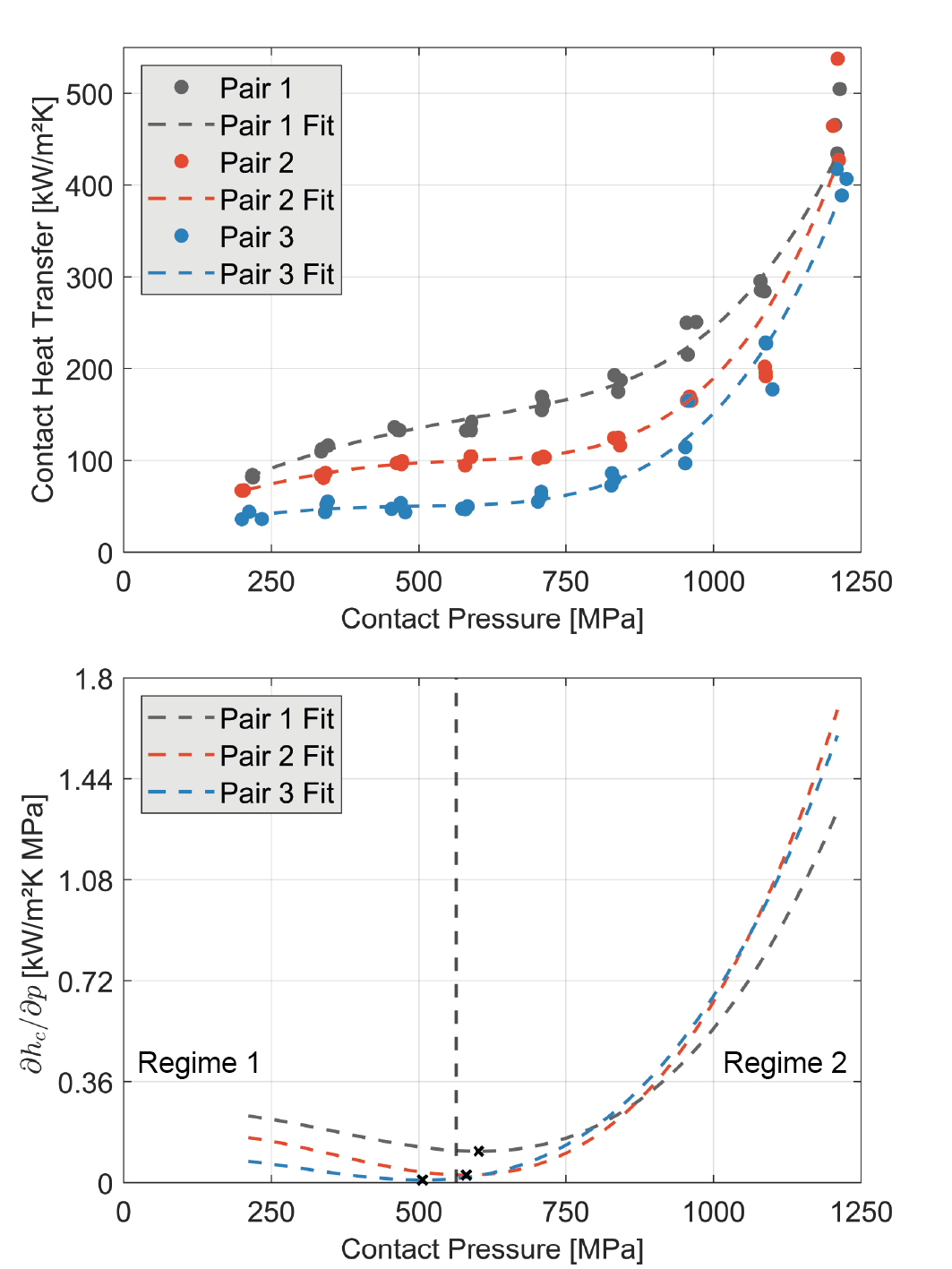
Bottom: Derivation of the contact heat transfer coefficient according to pressure for the two pairs of specimens as a function of pressure.
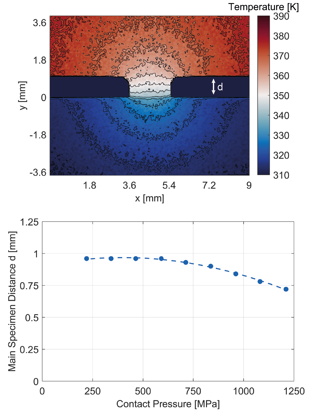
The individual measurement results for the respective sample pairing is consistent for itself over the measured pressure range. Nevertheless, it is observed that although the specimen pairs show the same qualitative trend, the contact heat transfer coefficient trend of pair 2 and 3 is significantly lower than the one of pair 1. Although the surface parameters are very similar, the microscopic contact points of the rough surfaces may be at different locations. The different contact conditions may be due to slight inaccuracies in the manufacturing of the specimens or the alignment of the specimens relative to each other in the experiment. This can lead to minor differences in the resulting heat-transferring interface and thus significantly affect the contact heat transfer coefficient. In the analytical correlations of Mikic and Cooper, the contact fraction AR/AN is equated with the ratio of contact pressure p and microhardness H by p/H. Here, the microhardness for C45 is 2000 MPa [17]. With reference to the observations in Figure 6, this means that at a contact ratio of 0.25 the transition from Regime 1 to Regime 2 occurs. It seems that starting from a contact ratio of about one quarter, the contact area is large enough that the thermal constriction in the contact plane is no longer so strong and the thermal resistance collapses. This parameter depends theoretically only on the material hardness and not on the roughness. This assumption must be confirmed in further experimental investigations. Due to the high pressures, both elastic and plastic deformations are expected in both test specimens. Figure 7 shows the macroscopic main specimen distance, which results from the height of the elevation, as a function of the contact pressure. This distance decreases by about a quarter from about 1 mm at 200 MPa to 0.75 mm at 1200 MPa. Visible deformation begins at about a contact pressure of 500 MPa, which agrees well with the magnitude of the yield strength of 510 MPa, above which plastic deformation occurs [18]. Although the elevation of the upper specimen is depressed, no widening is visible and the width of the elevation of 2 mm does not change. In the thermal simulation, pressure-dependent changes in the material properties due to plastic deformation have not yet been considered.
5. Conclusion
This paper presents a novel approach for inverse quantification of contact resistance under high loads using infrared thermography. The temperature information from the infrared images is used as input to the inverse optimization method, which aims to minimize between simulated and measured temperature by iteratively adjusting the sought thermal constraint. It is found that the thermal resistance collapses above a certain contact pressure or contact fraction and the heat transfer increases exponentially. Future studies will address the influence of different surface roughness and interstitial media in the contact zone on contact heat transfer. In the same way, the behavior of harder materials will be investigated. It will also be studied what is the main influencing factor causing the variation of the contact heat transfer coefficient of the different specimen pairings.
Acknowledgements
Mr. Göttlich and Mr. Gerhard would like to thank the Deutsche Forschungsgemeinschaft (DFG, German Research Foundation) for funding Project ID 422633203. Mr. Helmig gratefully acknowledges funding from the Deutsche Forschungsgemeinschaft Project ID 174223256-TRR 96.
References
[1] C. V. Madhusudana, "Thermal Contact Conductance", Berlin, Springer Science & Business Media, 2013.
[2] M. Cooper, B. Mikic, M. Yovanovich, "Thermal contact conductance", International Journal of heat and mass transfer vol. 12, no. 3, pp. 279-300, 1969. View Article
[3] B. Mikic, "Thermal contact conductance; theoretical considerations", International Journal of Heat and Mass Transfer, vol. 17, no. 2, pp. 205-214, 1974. View Article
[4] M. Asif and A. Tariq, "Correlations of Thermal Contact Conductance for Nominally Flat Metallic Contact in Vacuum", Experimental Heat Transfer, vol. 29, no. 4, pp. 456-484, 2016. View Article
[5] B. Sponagle, and D. Groulx, "Measurement of thermal interface conductance at variable clamping pressures using a steady state method", Applied Thermal Engineering, vol. 96, pp. 671-681, 2016. View Article
[6] D. Liu, Y. Luo, X. Shang, "Experimental investigation of high temperature thermal contact resistance between high thermal conductivity C/C material and Inconel 600", International Journal of Heat and Mass Transfer, vol. 80, pp. 407-410, 2015. View Article
[7] T. McWaid and E. Marschall, "Thermal contact resistance across pressed metal contacts in a vacuum environment", International Journal of Heat and Mass transfer, vol. 35, no. 11, pp. 2911-2920, 1992. View Article
[8] C. Fieberg and R. Kneer, "Determination of thermal contact resistance from transient temperature measurements", International Journal of Heat and Mass transfer, vol. 51, no. 5-6, pp. 1017-1023, 2008. View Article
[9] E.M. Burghold, Y. Frekers, R. Kneer, "Determination of time-dependent thermal contact conductance through IR-thermography", International Journal of Thermal Sciences, vol. 98, pp. 148-155, 2015. View Article
[10] O. Alifanov, "Inverse heat transfer problems", International Series in Heat and Mass Transfer, first ed. Springer, 1994. View Article
[11] J. V. Beck, B. Blackwell, C. R. S. Clair Jr, "Inverse heat conduction: Illposed problems", John Wiley & Sons Inc, 1985.
[12] M. M. Yovanovich, "Four decades of research on thermal contact, gap, and joint resistance in microelectronics", in IEEE Transactions on Components and Packaging Technologies, vol. 28, no. 2, pp. 182-206, 2005. View Article
[13] V. Kryzhanivskyy, R. M'Saoubi, J.-E. Ståhl, V. Bushlya, "Tool-chip thermal conductance coefficient and heat flux in machining: Theory, model and experiment", International Journal of Machine Tools and Manufacture, vol. 147, 2019. View Article
[14] V. Norouzifard, M. Hamedi, "Experimental determination of the tool-chip thermal contact conductance in machining process", International Journal of Machine Tools and Manufacture, vol. 84, pp. 45-57, 2014. View Article
[15] T. Helmig, T. Göttlich, R. Kneer, "An infrared thermography based experimental method to quantify multiscale thermal resistances at non-conforming interfaces", International Journal of Heat and Mass Transfer, 2021 View Article
[16] M. N. Ozisik, "Inverse heat transfer: fundamentals and applications", Crc Press, 2000.
[17] Y. Frekers, T. Helmig, E.M. Burghold, R. Kneer, "A numerical approach for investigating thermal contact conductance", International Journal of Thermal Sciences, vol. 121, pp. 45-54, 2017. View Article
[18] Calik, A., O. Sahin, and N. Ucar, "Mechanical properties of boronized AISI 316, AISI 1040, AISI 1045 and AISI 4140 steels.", Acta Physica Polonica A, vol. 115, no. 3, pp. 694-698, 2009. View Article