Journal of Fluid Flow, Heat and Mass Transfer (JFFHMT)

ISSN: 2368-6111

1. Introduction

This article is part of the industrial context of the development of electric vehicles, which require a Battery Thermal Management System (BTMS) for temperature control issues. Amongst a variety of solutions, the direct cooling of the pack immersed in a dielectric liquid circulating between the cells [1] is studied to prevent the thermal runaway propagation. The use of HFE-7100, which is a dielectric fluid, enables direct contact component cooling applications.

Confined boiling flow is a very efficient mode of heat transfer to dissipate high fluxes. Some papers present studies of convective flow boiling with HFE-7100 in vertical confined channels [2], [3]. To calculate heat transfer coefficient, these studies use inverse methods. Luciani et al. [3] show results with a predominance of nucleate boiling with local inverse method. Over the last two decade, the Eulerian two-phase CFD approach has gained in maturity to simulate boiling and dry out phenomena. Boiling is a complex phenomenon where both wall-fluid interaction and heat transfer have to be correctly taken into account for a suitable numerical approach. Chien et al. [4] compare an experiment and a CFD simulation of the flow boiling heat transfer coefficient of R410A in mini-channels.

In the present study, an experimental and a numerical study are jointly conducted to better understand, describe and quantify the boiling phenomenon of HFE-7100 in a vertical and rectangular mini-channel. Experiments are carried out from the onset of boiling to the dry-out occurrence, for different mass fluxes (G =140, 390 and 648 kg/(m².s)). An inverse conduction method has been developed to accurately estimate the experimental heat transfer. The approach includes Finite Difference Method for the modeling and a Tikhonov's method for the regularization. The impact of different mass flow rates on boiling and dry-out occurrence is observed and measured.

A CFD approach is then proposed and validated on these experimental data, in the view to propose a boiling model of the flow, including the mesh, which aims to be general enough to be extrapolated to an entire system, for example a battery pack. Consistently, the flow is numerically modelled in this paper within a vertical 2D channel approach, which is directly extendable to 3D. This modelling aims to predict, over the entire operating range of an experimental device, the value of the various quantities of interest such as the void fraction, the heat transfer coefficient and the temperature at the wall.

2. Description of the experiment

2. 1. Experimental facility

The aim of the experiment is to provide data for pure HFE-7100 convective flow boiling analysis with heat transfer measurements. The loop has the function to supply to the test section the required wall heat power, HFE-7100 flowrate and fluid temperature.

As shown in Figure 1, the loop is a closed circulation of the HFE-7100, which is the working fluid, cooled by an external circulation of water. The working fluid flows successively through the following components: a gear pump; a Coriolis mass flowmeter; a pre-heater; a test section; a condenser; a compensating tank. The pressure in the test section is controlled by a thermo-regulated tank.

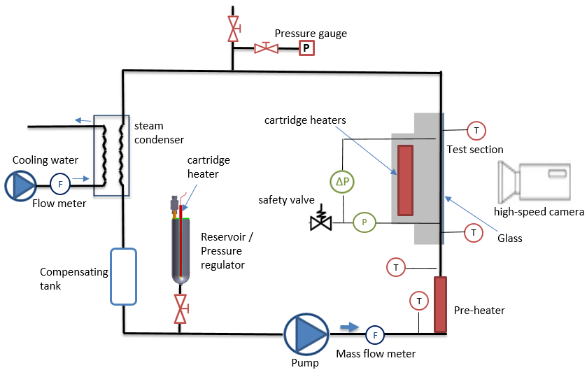
The main element of the experimental device is the test section (Figure 2 and Figure 3), composed of a vertically oriented mini-channel.

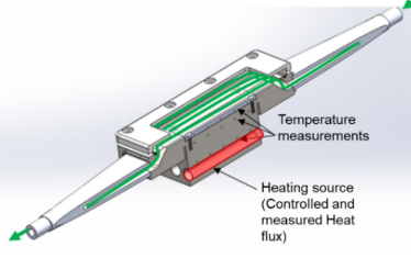
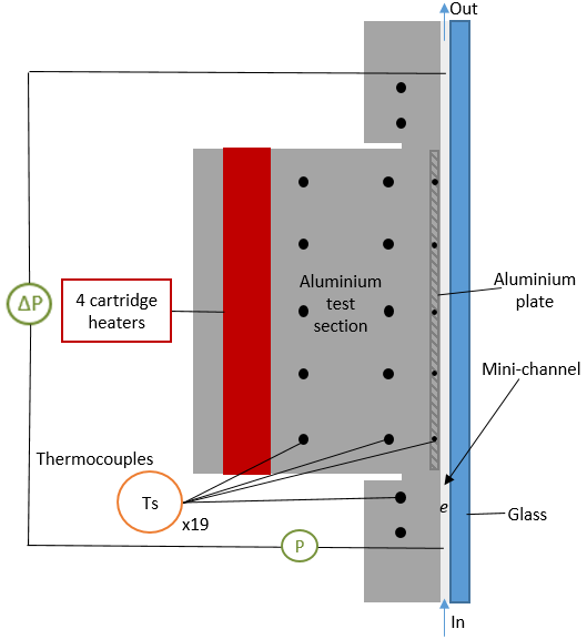
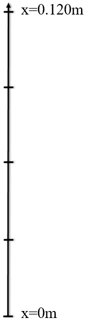
The device is a 1mm deep, 30mm wide and 120mm long rectangular channel. The heat flux is set on 80mm long. The test section is made of aluminum 6061. A part of the wall is a plate, made of the same material, inserted and fixed. A graphite paper achieves the thermal contact. Four heating cartridges of 600W max each heat the test section and the heat transfer produced is transferred by heat conduction to the fluid. The test section includes three rows of five K-type thermocouples (TC) each, including one row within the plate, which serves as a measurement for the channel wall. Along the channel, a distance of 15mm separates each thermocouple from its neighbors. Two pressure sensors at the mini-channel inlet and outlet measure the average pressure in the test section. The fluid saturation temperature T_sat of the fluid is deduced from pressure measurement. The test section is thermally insulated.

2. 2. Experimental Procedure

The tests are carried out at a fixed and constant flow rate. The inlet pressure of the mini-channel is controlled to be kept constant at approximately 1.1 bar (saturation temperature of 64°C). The inlet temperature of the test section is adjusted at 60°C. For three fixed mass fluxes (G =140, 390 and 648 kg/(m².s)), the heat flux set by the heating cartridges is increased step by step from the onset of boiling (1 W/cm²) to the wall dry-out (wall superheat  of about 100°C, 20W/cm²).

The uncertainties of the different quantities measured in this study are presented in Table 1.

Table 1. Uncertainties of the measured parameters.

Experimental parameter	Maximum absolute error
Temperature of the section	1K
Absolute pressure	20 mbar (2000 Pa)
Mass flow rate G	0.32kg/h
Pressure drop	0.5 mbar (50 Pa)

2. 3. Experimental data reduction by 2D inverse method

A numerical method is detailed in this section and in a previous paper [5], with the aim to accurately calculate the local heat transfer coefficient at the heated wall of the mini-channel, relying on the temperature measurements. For the calculations of the local heat transfer coefficient, it is assumed that the fluid temperature is equal to the mean saturation temperature T_sat throughout the channel. Measurements and calculations are both carried out in a steady state.

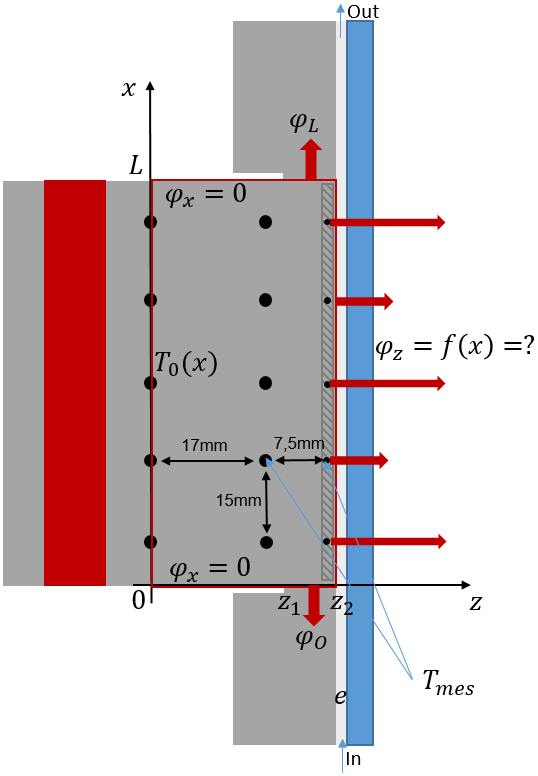
The principle of this method is that it is possible to deduce unknown boundary conditions such as the heat flux from a known part of the temperature field. The problem is schematically described in Figure 4. It is assumed to be two-dimensional in (x, z) directions.

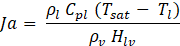
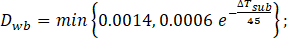
The experimental local heat transfer coefficient h_exp is calculated along the vertical channel wall according to the following equation:

(1)

(2)

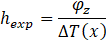
where φ_z is the heat flux, at the wall, in the z direction and ∆T(x) the wall superheat, T_w(x) is the wall temperature measured by the TCs in the plate and T_sat the mean saturation temperature.

Firstly, the fundamental equations are written in the solid domain. Since the problem is purely conductive, it is governed by the 2D heat equation:

(3)

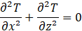
where T is the temperature and (x,z) the directions.

The Boundary conditions are described below and shown in Figure 4. On the z=0 line, the Dirichlet condition T₀(x) is known: it is a “makima” [6] interpolation in the x direction of measured temperatures at TCs locations.

On both other lines of TCs, using the same “makima” interpolation, T(x) is then further considered as known, and is further called T_mes. The objective of the following outlined inverse method is to calculate the total heat flux φ_Tot=(φ_L φz φ_o)) knowing T_mes which is the measured temperatures at TCs locations.

Secondly, the system of equations are spatially discretized with a finite difference method, as described in [7], and written in matrix form. The matrix system must be modified and decomposed to obtain a linear relation between T_mes and the unknown boundary condition φ_Tot as follows:

(4)

where S is the so-called sensitivity matrix. Next, the system must be inversed and solved.

(5)

The regularization of the matrix is carried out by the Tikhonov penalization technique. The system is solved for different values of Tikhonov regularization coefficient μ introduced in the equation as follows:

(6)

where R is chosen as the identity matrix. The best solution is found when the difference between the measurement and the model ‖S*φ_Tot-T_mes‖² is at its minimum value in a numerically stable region, using the L-curve technique [8].

3. Numerical approach

3. 1. Set-up of the test case

A 2D planar geometry of part of the test section with the vertical mini-channel is modelled in ANSYS Fluent and presented in Figure 5. The mini-channel has a total length of 140mm, (to take into account the heat diffusion upstream and downstream of the channel) and a studied length of L=80mm. The width l, equal to 30 mm, is specified in the software in order to work with the same mass flow values as in the experimental setup. The deep e is equal to 1mm.

The channel mesh is composed of 5 radial and 32 axial cells on the heated part L and has been chosen relatively coarse on purpose, in view of a 3D extension to a system which length scale is several order of magnitude larger than the mini-channel, for example a battery pack. In addition, a mesh sensitivity study was performed, and showed no significant change in the results for a mesh size two times finer.

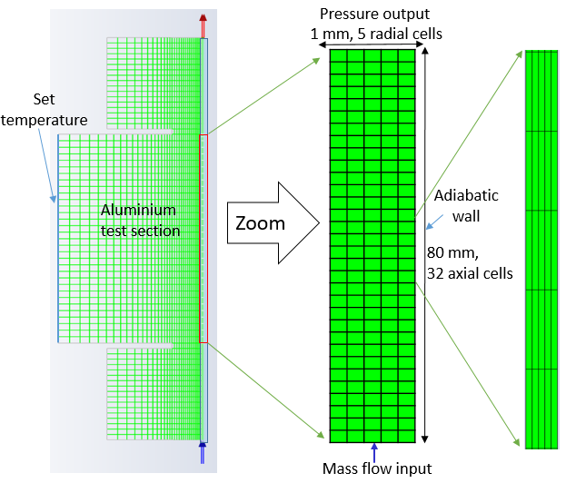
The problem is treated in steady state. The mass flow rate is defined at the channel inlet. The HFE-7100 enters the liquid phase at a temperature of 333.81 K, i.e. a subcooling of 3.01 K; the channel outlet is specified at constant pressure. The outer wall of the channel is defined as "adiabatic wall". The "heated wall" at the first row of thermocouples is set as the imposed temperature.

Physical properties of HFE-7100 in the liquid and vapor phase are determined from the EES software database, presented in Table 2 and entered to Fluent. The properties of HFE-7100 in the liquid state are defined as constant between the inlet temperature 333.81K and the saturation temperature 336.82K. The properties of HFE-7100 in the vapor state are given at the saturation temperature (T_sat= 336.82 K) of HFE-7100 at 1.1 bar. The liquid state is defined as the main phase of the two-phase flow.

Table 2. Physical properties of liquid and vapor (saturated) HFE-7100.

phase	liquid	vapor
T (K)	333.81	336.82
(kg.m-3)	1 422	9.571
Cp (J.kg-1.K-1)	1177	937.7
k (W. m-1. K-1)	0.06199	0.008604
(kg.m-1.s-1)	3.97 10-4	1.986 10-5
M (kg.kmol-1)	250	250
H (J.kgmol-1)	6.83171.107	9.72329.107
(N/m)	0.009596

3. 2. Two-fluid model

In the present study, the two-fluid model called Euler-Euler approach is used to calculate the two-phase flow. The 6 equations are solved, each phase being described by the 3 conservation equations. The equations are provided by the theory guide of Fluent [9].

The Critical Heat Flux model (CHF) is an extension of the RPI [10] wall boiling model; it takes into account the rise in temperature of the vapor, unlike the RPI model in which the vapor temperature is assumed to be constant. The decomposition of the heat flux at the wall is expressed as:

(7)

where the different heat flux and function f(α_l) are defined in the following equations.

The convective heat flux with the liquid phase is expressed as:

(8)

with h_c the liquid phase heat transfer coefficient, T_w the wall temperature, T_l the liquid temperature and A_b the area of influence.

The quenching heat flux models heat transfer occurring when the liquid fills the wall vicinity after bubble detachment is expressed as:

(9)

with k_l the liquid heat conductivity, ρ_l the liquid density, C_pl the liquid phase specific heat and T the periodic time. The quenching model correction is used with the y+ value fixed to 250 as default.

The evaporation heat flux is equal to:

(10)

with D_wb the bubble departure diameter, N_w the nucleate site density, ρ_v the vapor density, H_lv the latent heat of evaporation, f the frequency of bubble departure.

The vapor convective flux is expressed as:

(11)

with h_v the vapor phase heat transfer coefficient and T_v the vapor temperature.

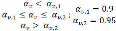
The function f(α_l) depends on the local liquid / vapor volume fraction α_l / α_v. The expression of Tentner et al. [11] is used.

for;

(12)

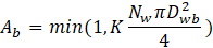
The area of influence A_b is defined as the fraction of the wall covered with forming vapor bubbles. The area of influence is determined from the bubble departure diameter and the nucleation site density:

(13)

The empirical constant K is calculated by Del Valle and Kenning [12]:

(14)

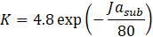
with Ja_sub the subcooled Jacob number. It is defined as:

(15)

The bubble departure diameter is calculated from the correlation of Tolubinski & Kostanchuk [13] :

(16)

The frequency of bubble departure is based on inertia controlled growth by Cole [14]:

(17)

where g is the gravity acceleration.

Nucleate site density is estimated by Lemmert and Chawl correlation [15]:

(18)

where n=1.41 and C=220, which are the values recommended by ANSYS support [Private Communication] to get the CHF model consistent with the RPI one in the nucleate regime.

The turbulence model k-ε RNG, with the near-wall treatment "Non Equilibrium Wall Functions", is used. Two forces are taken into account to model interfacial transfers. To evaluate the different interfacial transfers between the two phases, the interfacial area concentration has been determined using the particle model. In this study, only the turbulent dispersion and the drag force are considered.

The turbulent dispersion force is determined using the original model of Lopez de Bertodano [16], with a turbulent dispersion coefficient C_TD=1.

The interfacial drag force is computed using the drag coefficient C_D from Ishii-Zuber model [17].

The turbulent interaction, i.e. the turbulence source term induced by the secondary phase, is determined by the Troshko-Hassan model [18].

4. Results and Discussion

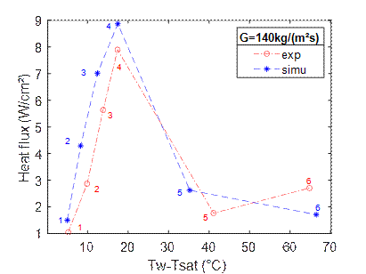
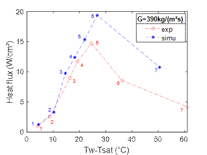
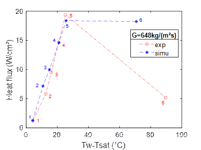
Figure 6 compares the experimental and numerical boiling curves. Boiling curves represent the heat flux versus wall superheat (Tw-T_sat), at three different mass flow rates (140 kg/(m².s); 390 kg/(m².s); 648 kg/(m².s)) at the wall central axial location.

On the boiling curves, the critical heat flux (CHF) is the maximum heat flux before the dry-out, which is characterized by the inflexion of the curve due to a strong increase in wall temperature. On the one hand, the heat transfer of HFE-7100 increases with the increase of the heat flux. On the other hand, there is a small impact of the mass flow rate on the heat transfer coefficient. Both points suggest a significant influence of the nucleate boiling mechanism on the heat transfer.

CFD simulations for several points and for the three mass flows rates correctly predicts experimental heat transfer coefficients before dry-out. The dry-out occurrence and the value of the CHF are also well predicted, at 140 kg/(m².s) (a) and 648 kg/(m².s) (c). For the mass flow rate of 390 kg/(m².s) (b), the CFD overestimates the value of the heat flux at the peak (point 6) characteristic of the CHF, which by the way happens earlier in the experiment (at point 5). An explanation of the difference in the occurrence of the dry-out between the CFD and the experiment is the local representation of the boiling curve. Indeed, the boiling curve is plotted at the central axial position of the channel. Therefore, a better understanding of the difference between the CFD and experimental value on point 6 is provided by the following axial profile (Figure 7 (e)).

The difference of heat flux, after dry-out, for G=390 kg/(m².s) (b) and 648 kg/(m².s) (c), can be explained by an adiabatic condition which is less true in the experiment at high temperatures than in CFD where the boundary condition is mathematical. The explanation would be that despite the overheating of the wall, a large flux is transferred to the fluid to respect the energy balance.

(a)
(b)
(c)

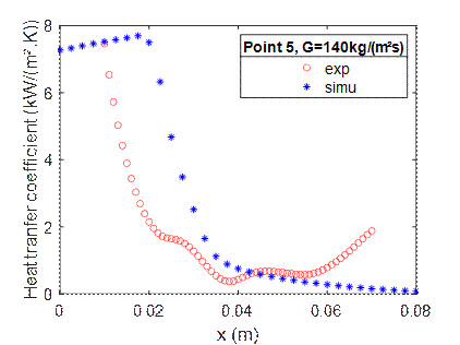
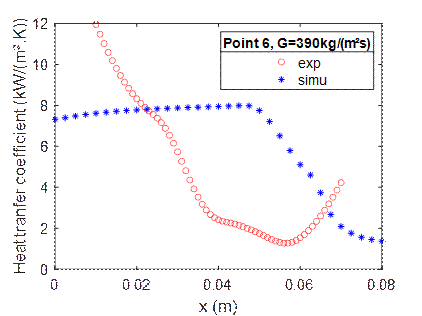
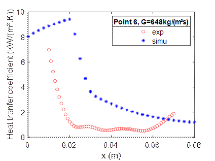
Figure 7 shows the CFD and experimental comparison of the heat transfer coefficient (HTC) profile along the channel for different points, at the three mass flow rates.

The abrupt rise of the experimental heat transfer coefficient downstream of the channel is due to the edge effect caused by the axial heat loss in the test section. This edge effect will be further investigated.

For the axial profile of the HTC at G=140 kg/(m².s) and point 5 (d), which corresponds to a state where the dry out has already occurred, the order of magnitude of HTC before and after the dry-out is similar between the CFD and the experiment. The CFD dry-out appears at an axial position relatively close to the experiment.

The selected point 6 at G=390 kg/(m².s) (e) corresponds to a state where the dry-out occurred at x=0.04m for the experiment whereas it occurs at x=0.06m for the CFD. This result explains the difference between the CFD and the experiment in point 6 of the boiling curve (Figure 6). Nevertheless, the order of magnitude of HTC before and after the dry-out is similar between the CFD and the experiment.

Plot (f) is the comparison of the CFD and experimental axial profile of the HTC at G=648 kg/(m².s), and shows a dry-out that occurs at almost the same axial position.

The heat transfer and the dry-out occurrence in CFD calculations are sensitive to some parameters of the closure laws. The Tentner et al. [11] blending function f(α_l ) of Eq. (12) which has been used, with the α_v,1 and α_v,2 parameters by default, for the CFD validation, has an important impact on the dry-out occurrence. These parameters can be adjusted to delay or advance the onset of dry-out. In addition, some parameters such as the area of influence A_b in Eq. (8) and Eq. (9) and the bubble departure diameter D_wb in Eq. (10) have an impact on both heat transfer and dry-out occurrence. The empirical constant K in Eq. (14) calculated by Del Valle and Kenning [12] and the correlation of Tolubinski & Kostanchuk [13] in Eq. (16)) can also been mentioned.

All these closure laws parameters use experimental correlations or have been more or less directly determined and validated on the basis of different experimental data than the present ones: different fluid (generally water) and conditions. However, they are used in their original form in the present simulations, without specific tuning, which makes these calculations rather of a blind type. Thereafter, an improvement of the CFD closure laws parameters fitting to the experimental tests may be considered in further studies but it is out of the scope of the present paper. Moreover, for future use in simulations of thermal runaway of a battery pack immersed in HFE7100, the present work simulation versus experiment consistency has to be evaluated with regard to uncertainties about the scenario of a battery cell thermal runaway within a battery pack. These uncertainties are about the energy release, the amount and composition of ejected gas [19], the amount and diameter distribution of ejected solid particles [20].

(d)
(e)
(f)

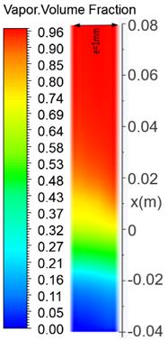
Figure 8 shows the contour of the calculated vapor volume fraction. The simulated results is obtained with mass flow rate G=140 kg/(m².s), at point n°5 (at dry-out). At this flux level, the vapor volume fraction increases rapidly along the mini channel. The vapor volume fraction increases from 0.2 to 0.8 between "-0.02m" and 0.02m. It can be seen that it is rather homogeneous in the depth e=1mm of the mini channel.

5. Conclusion

The experimental heat transfer coefficient of HFE-7100 flow boiling in a vertical mini-channel was deduced from measurements associated to an inverse method resolution. The experimental results show that the heat transfer coefficient is strongly dependent on the heat flux but weakly dependent on the mass flux, which suggests a significant influence of the nucleate boiling mechanism on the heat transfer. An Eulerian multiphase multi-D approach with a Critical Heat Flux wall-boiling model has been validated with the experimental results. The comparison has been carried out from the onset of boiling to dry-out, for three mass fluxes, with satisfactory results. The numerical simulation shows a satisfactory prediction of the experimental heat transfer coefficients and the dry-out occurrence.

References

[[1] M. Suresh Patil, J.-H. Seo, and M.-Y. Lee, "A novel dielectric fluid immersion cooling technology for Li-ion battery thermal management," Energy Convers. Manag., vol. 229, p. 113715, 2021. View Article
[[2] M. Piasecka, K. Strąk, and B. Maciejewska, "Heat transfer characteristics during flow along horizontal and vertical minichannels," Int. J. Multiph. Flow, vol. 137, p. 103559, Apr. 2021. View Article
[3] S. Luciani, D. Brutin, C. Le Niliot, L. Tadrist, and O. Rahli, "Boiling heat transfer in a vertical microchannel: local estimation during flow boiling with a non intrusive method," Multiph. Sci. Technol., vol. 21, no. 4, Art. no. 4, 2009. View Article
[4] N. B. Chien, K.-I. Choi, and J.-T. Oh, "Experiment and CFD Simulation of Boiling Heat Transfer Coefficient of R410A in Minichannels," Int. J. Air-Cond. Refrig., vol. 23, no. 04, 635845248000000000. View Article
[5] R. Lioger-Arago, P. Coste, and N. Caney, "Study of flow boiling in a vertical minichanel: heat transfer analysis using inverse method," presented at the 15th HEFAT-ATE International Conference, 2021.
[6] "Modified Akima piecewise cubic Hermite interpolation - MATLAB - MathWorks France."
[7] D. Maillet, Y. Jarny, and D. Petit, "Problèmes inverses en diffusion thermique - Formulation et résolution du problème des moindres carrés," Ref: TIP201WEB - "Physique énergétique," Jul. 10, 2018. View Article
[8] [8] P. C. Hansen, "Rank-Deficient and Discrete Ill-Posed Problems: Numerical Aspects of Linear Inversion," 1998. View Article
[9] Ansys Fluent, 2021 R2, "Theory Guide."
[10] N. Kurul and M. Z. Podowski, "On the modeling of multidimensional effects in boiling channels," In Proceedings of the 27th National Heat Transfer Conference, Minneapolis, Minnesota, USA, 1991.
[11] A. Tentner, S. Lo, and V. Kozlov, "Advances in Computational Fluid Dynamics Modeling of Two-Phase Flow in a Boiling Water Reactor Fuel Assembly," In International Conference on Nuclear Engineering, Miami, Florida, 2006. View Article
[12] V. H. Del Valle and D. B. R. Kenning, "Subcooled flow boiling at high heat flux," International Journal of Heat and Mass Transfer, 1985. View Article
[13] V. I. Tolubinski and D. M. Kostanchuk, "Vapor bubbles growth rate and heat transfer intensity at subcooled water boiling," 4th International Heat Transfer Conference, Paris, France, 1970. View Article
[14] R. Cole, "A Photographic Study of Pool Boiling in the Region of the Critical Heat Flux," AIChE J., 1960. View Article
[15] M. Lemmert and L. M. Chawla, "Influence of flow velocity on surface boiling heat transfer coefficient in Heat Transfer in Boiling," E. Hahne and U. Grigull, Eds., Academic Press and Hemisphere, New York, NY, USA, 1977.
[16] M. Lopez de Bertodano, "Turbulent Bubbly Flow in a Triangular Duct," Ph.D. Thesis, Rensselaer Polytechnic Institute, Troy, New York, 1991.
[17] M. Ishii and N. Zuber, "Drag Coefficient and Relative Velocity in Bubbly, Droplet or Particulate Flows," AIChE J., 1979. View Article
[18] A. A. Troshko and Y. A. Hassan, "A Two-Equation Turbulence Model of Turbulent Bubbly Flow," International Journal of Multiphase Flow, 2001. View Article
[19] S. Koch, A. Fill, and K. P. Birke, "Comprehensive gas analysis on large scale automotive lithium-ion cells in thermal runaway," J. Power Sources, vol. 398, pp. 106-112, Sep. 2018. View Article
[20] V. Premnath, Y. Wang, N. Wright, I. Khalek, and S. Uribe, "Detailed characterization of particle emissions from battery fires," Aerosol Sci. Technol., vol. 0, no. 0, pp. 1-18, Dec. 2021.