Journal of Fluid Flow, Heat and Mass Transfer (JFFHMT)

ISSN: 2368-6111

1. Introduction

In an automotive paint shop, the BIW passes through various stages of applying paint coats and treatments. One of the most critical stages is the Electro-dip coating or ED-coating. It is a process of electrically applying anti-corrosion coatings on the BIW and other automotive parts. Since its inception in the early 1960s, electro-dip process has evolved, and its operational efficiency has improved. Some of the aspects driving its development are (a) aesthetics and quality; (b) improved corrosion protection; (c) speed of assembly line; (d) reducing environmental impact; (e) cost; (f) durability [1]. The first processes of dip coating were based on anodic electrodeposition where the BIW acted as the anode. However, driven by higher process efficiency and reliability offered by cathodic deposition which were introduced in mid-1970s, adoption of cathodic electrodeposition increased [1]. E-coating offers excellent adhesion to metal and high resistance to displacement by water [2].

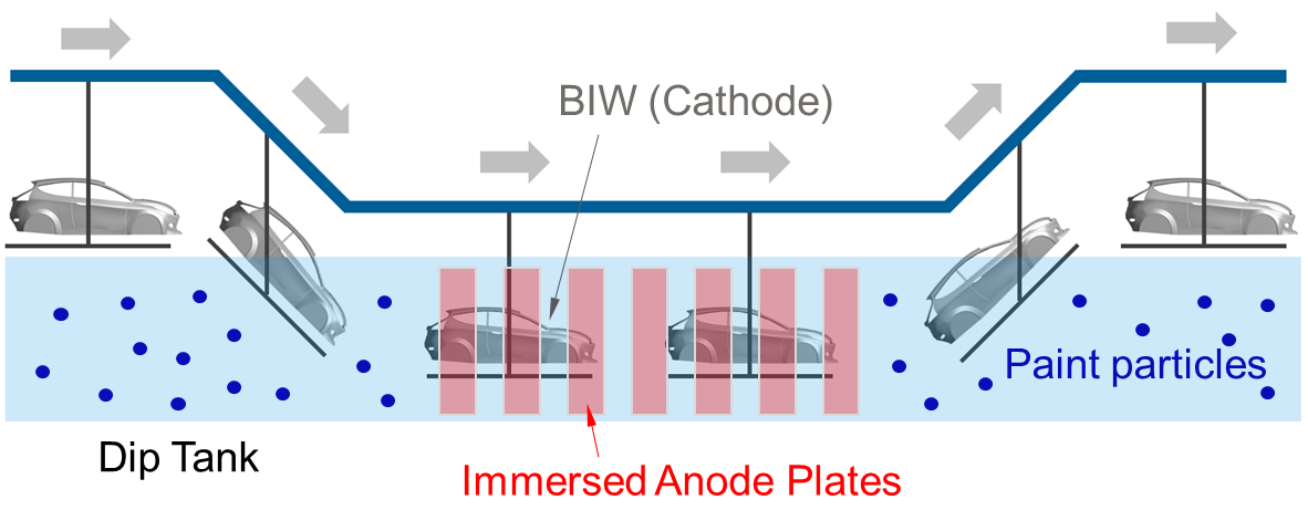
The e-coat process is schematically shown in Figure 1. Paint particles are dispersed in water held in an immersion bath, which is also called as the dip tank or ED-tank. The process starts by dipping the automotive BIW into the ED-tank. In cathodic electrodeposition process, the BIW acts as the cathode. Anode plates are lined up along the walls of the tank. Positively charged paint particles are attracted by and deposited onto the BIW. The thickness of the coat can be regulated by the applied voltage, operating temperature, tank residence time, and concentration of paint particles in the coat solution [3]. As compared to a spray paint process, the dipping ensures a better reach of paint particles on the inner BIW skin, holes, interior cavities, especially those on pillars and sills of the BIW. The coated BIW is further heat treated in a downstream curing oven, resulting in an insoluble deposited layer with very strong adherence to the pre-treated BIW surface [4].

Automotive industry is constantly faced with challenges to improve its manufacturing processes, reduce costs, improve quality, while meeting the emission and environmental policies. Further, shortened timelines for new product development cycles demand reduced prototype testing. Therefore, automotive OEMs are increasingly relying on CAE, virtual testing, and simulations to make faster and smarter design decisions and reduce physical tests. Automotive paint shop processes are no exception and utilize simulations in various stages of a paint shop from pre-coating treatments to e-coating to oven curing processes [5]. Since paint shop is responsible for the highest energy consumption in the production process [6] and its processes affect the overall durability, corrosion and chip resistance of the car body, simulations are used to address and aid different aspects of the process. E-coating can suffer from defects like uneven deposition, zero to very low thickness deposition on interior cavities due to air entrapment, which are typically identified late in the prototyping stage by tearing the BIW apart. Therefore, simulations can be applied in the early stages of the design and prototyping to save costs and time.

In this study, a simulation methodology is presented using Ansys Fluent to predict two aspects of an electro-dip process which directly affect the paint deposition quality and costs,

1. Air entrapment: During the dip-in process, air bubbles may get trapped in certain locations of the BIW resulting in lack of paint deposition and/or reducing the paint contact time.
2. Carryover of residual paint: During the dip-out process, paint drains at a rate controlled by the size of holes and drain paths. Liquid residue that gets carried over to the successive baths affects the process quality and affect the drying process [5].

Therefore, the proposed methodology can aid in the identification of critical areas subjected to air entrapment and reduce paint carryover early in the product design cycle, thereby improving the process design, product quality, and saving costs from late design changes.

2. Electro-dip Motion Profiling

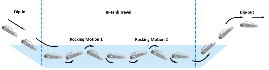
The first step in performing the e-dip simulation is to obtain the BIW motion profile in terms of translational and rotational components along the x, y, z directions. The motion considered in the present study is shown schematically in Figure 2. Dip-in motion is followed by two rocking movements with intermediate straight travels.

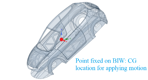
BIW geometry used in this study and the point fixed on the BIW to which the motion is applied is shown in Figure 3 (a). Path followed by this point during the entire dip motion is shown in Figure 3 (b).

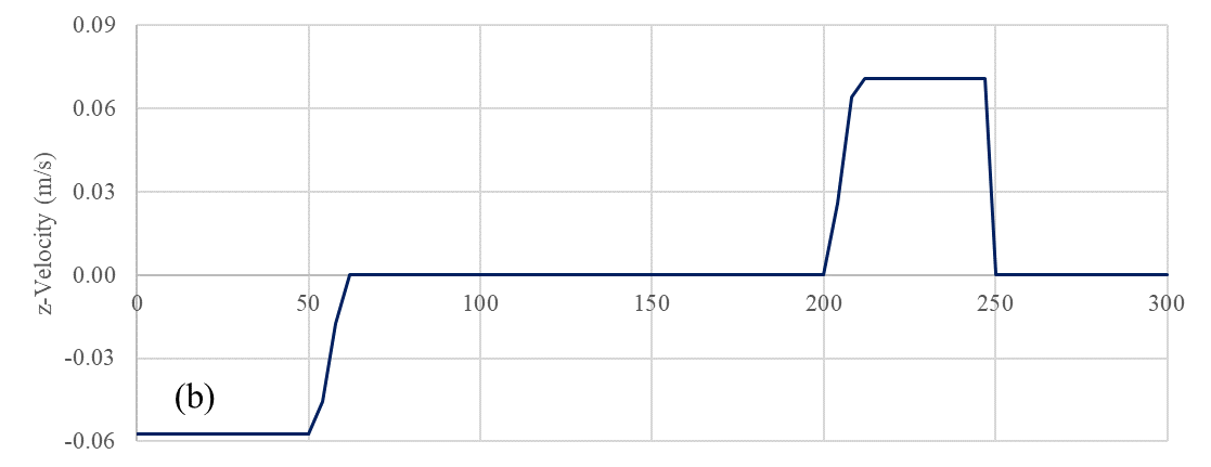
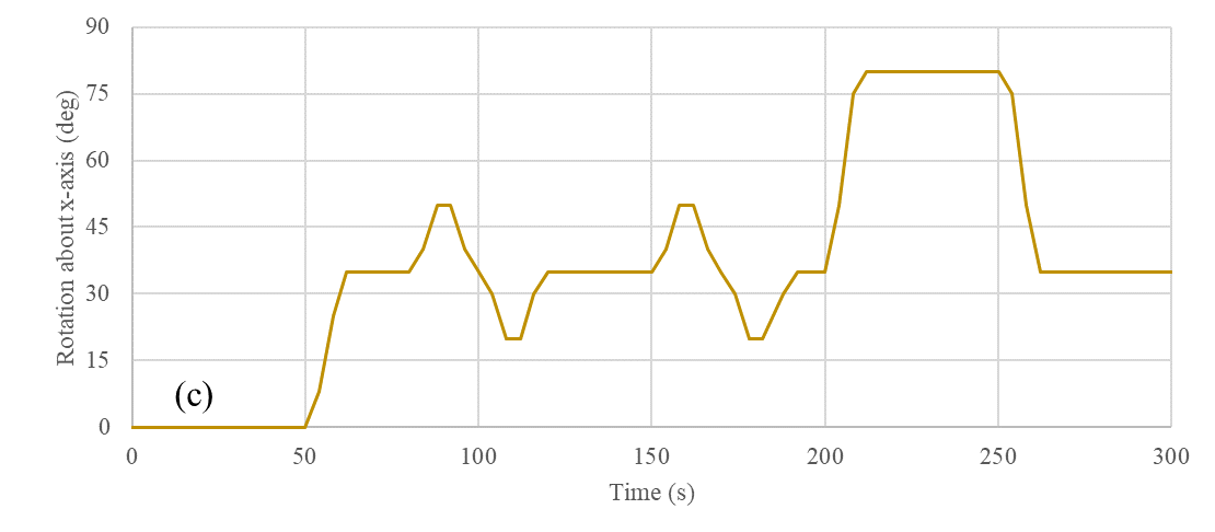
The temporal variation of travel velocities and angular orientation of the BIW that represents the rotational motion are shown in Figure 4. These profiles serve as inputs to the dynamic mesh motion methods used in Ansys Fluent.

(a)
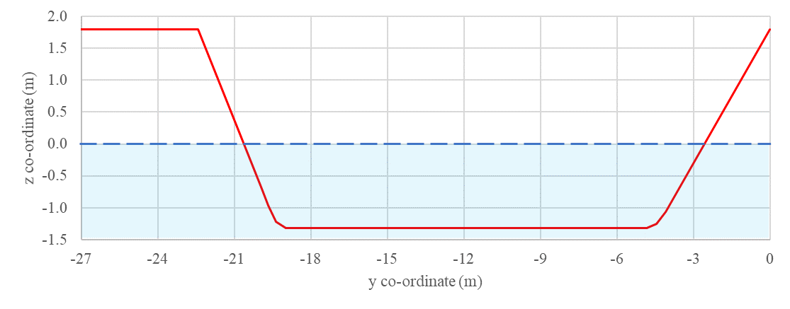(b)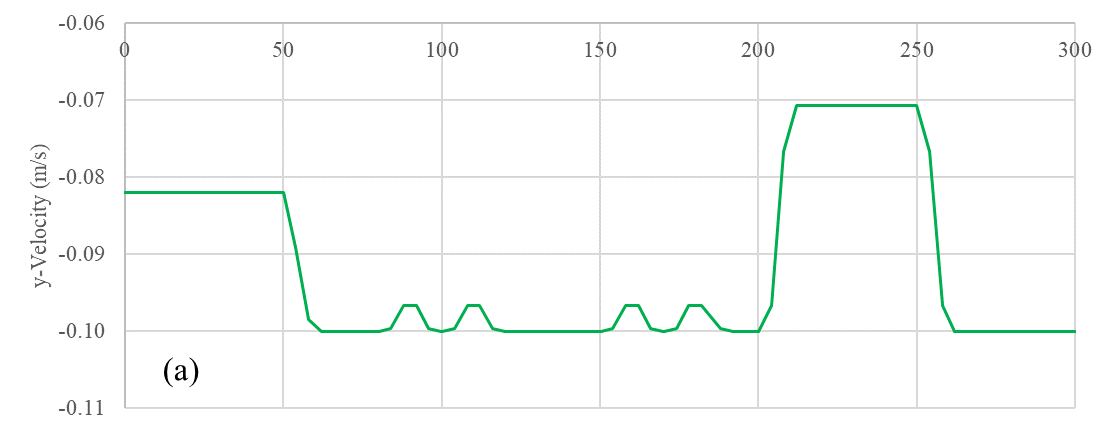

3. Overview of the Multiphase Model

Finite volume method (FVM) with the pressure-based solver implemented in the commercial code Ansys Fluent is used to solve the flow equations. Two-phase free surface flow between air and liquid paint is modelled using the Volume of Fluid (VOF) Method which can accurately capture the interface between immiscible fluids. Mesh motion is implemented using Rigid Body motion and Dynamic Mesh Layering techniques.

3. 1. Governing Equations

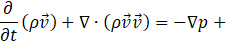
The VOF model can model two or more immiscible fluids by solving a single set of momentum equations and tracking the volume fraction of each of the fluids throughout the domain. The fluid properties are represented by volume-averaged values. The variables and properties in any given cell are either purely representative of one of the phases, or representative of a mixture of the phases, depending upon the volume fraction values. For example, if the q^th fluid’s volume fraction in the cell is denoted as α_q, then (a) α_q = 0: absence of q^th fluid in the cell, (b) α_q = 1: cell is fully filled with the q^th fluid, and (c) 0 < α_q < 1: cell is partially filled with q^th fluid and contains the phase interface. [7]

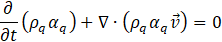
The tracking of the interface(s) between the phases is accomplished by the solution of a continuity equation for the volume fraction of one (or more) of the phases. For the q^th phase in absence of mass transfer, this is given by Eq. (1). Volume fraction equation will not be solved for the primary phase; since it is computed based on the constraint given by Eq. (2).

(1)

(2)

Volume fraction equation is solved using the implicit formulation in this study. A single momentum equation is solved over the domain, as given by Eq. (3).

(3)

where ρ and μ are volume-weighted averaged properties, represents the surface tension force at the interfaces.

3. 2. Volume Fraction Discretization using the Sharp/Dispersed Compressive Scheme

In the volume fraction equation, face values of volume fraction used in the convection term are discretized using a modified compressive scheme available in Ansys Fluent which is a second-order reconstruction scheme based on slope limiters [7]

(4)

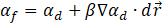
where α_f = face VOF value, α_d = donor cell VOF value, β = slope limiter value, ∇α_d = donor cell VOF gradient value, and = cell to face distance

3. 3. Surface Tension and Wall Adhesion Effects

Continuum surface force (CSF) model which accounts for surface tension between a phase pair as a continuous, volumetric body force term is applied in this study. It has the following form:

(5)

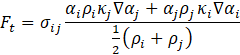
where curvature , interface unit normal . Effects of wall adhesion at the BIW surfaces is also incorporated within the CSF model framework. The contact angle specified at the walls is used to adjust the surface normal in cells near the wall. If θ_w is the contact angle at the wall, then the surface normal at the cell next to the wall is given by Eq. (6).

(6)

where and are the unit vectors normal and tangential to the wall, respectively. The combination of this contact angle with the normally calculated surface normal one cell away from the wall determine the local curvature of the surface, and this curvature is used to adjust the body force term in the surface tension calculation.

4. Overview of the Solution Approach

Ansys Fluent offers Dynamic Mesh and Overset Mesh Motion techniques to incorporate relative motion between zones. In this study, a dynamic mesh approach combined with relative paint motion is employed to capture the e-dip process. Domain decomposition and computational mesh generated to achieve this is discussed here.

4. 1. Pre-processing

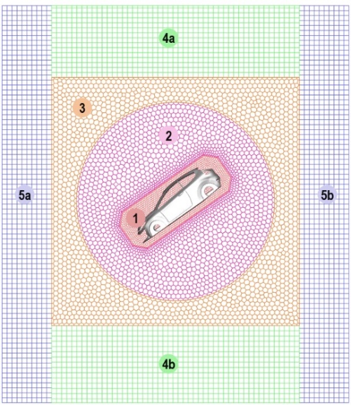
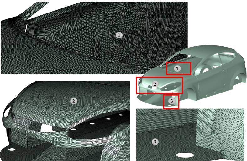
The simulation domain used in this study is shown in Figure 5(a). It is decomposed into several zones to facilitate the application of mesh motion that mimics the e-dip motion profile. Zone 1 encompasses the BIW body and was decomposed from zone 2 to allow a refined volume mesh near the region of interest. Zone 2 is a cylindrical domain centred about the fixed point on BIW which is used as the CG location for applying motion (refer Figure 3(a)). Zone 3 encloses the cylinder to form planar interfaces with the outer zones 4 and 5. Polyhedral mesh is generated in zones 1, 2 and 3. Surface mesh size on the BIW in zone 1 is maintained between 1 to 8 (mm). Two prism layers are generated on the car body using an aspect ratio of 5 for the first layer. The maximum element size is set as 80 (mm) in zone 1. It transitions to a maximum element size of 200 (mm) in zone 2. Zone 3 is also meshed with a polyhedral mesh having an element size of 200 (mm). The other zones are meshed with hexahedral elements of 200 (mm). The total mesh count of the domain is about 4.7 million.

4. 2. Mesh Motion Technique

BIW motion can be decomposed essentially into three components: (a) horizontal translation, (b) vertical translation, and (c) angular orientation; refer Figure 4. The methodology proposed in this study employs the following motions zone-wise:

1. Zones 1 and 2 undergo vertical translation + rotational rigid body motion
2. Zone 3 is subjected to a vertical motion only
3. As the zones 1, 2 and 3 translate vertically, zone 4 undergoes Dynamic Layering to accommodate the relative motion between its boundary surface zones. For example, during the downward motion of BIW, layers get removed in zone 4b and new layers get added in zone 4a.

While mesh motion is used to account for vertical and rotational components of the dip motion, horizonal component gets applied through relative paint velocity supplied via the flow boundaries.

4. 3. Boundary Conditions

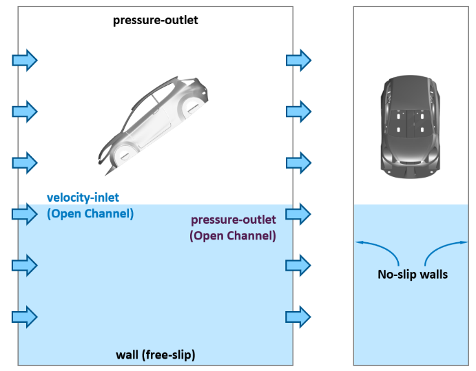
Open channel wave boundary conditions are available within the VOF model framework in Ansys Fluent. They facilitate the setup of hydrostatic pressure gradients and free surface levels at the inlet and outlet boundaries, as shown in schematic Figure 6.

At the open channel inlet boundary, the y-velocity is specified based on the transient profile shown in Figure 4(a). It must be noted that the velocity shown in Figure 4(a) represents the actual motion component of the BIW. Since the paint velocity must be applied in the reverse direction of the actual horizontal motion component, the profile is multiplied with a -1 before applying at the inlet boundary. At the open channel outlet boundary, atmospheric pressure is applied. The top bounding surface of the domain is also considered as a pressure-outlet boundary open to atmospheric pressure. The bottom surface is considered as a zero-shear or a free-slip wall.

While implementing the mesh motion technique, one of the assumptions implicit in the approach is that the effect from the lower bounding wall of the tank is neglected. Therefore, the lower extent of the domain does not correlate with the physical depth of the tank. This is valid since the bubble escape and trapping is not governed by the bottom surface. This assumption is supported through the comparison of predictions using the Overset Mesh motion technique with the proposed method and is presented later in this paper.

4. 4. Material Properties

Material properties used in the computational model are given in Table 1. Paint properties are assumed to be that of water at 30 0C. Air density is assumed to be based on ideal-gas law with temperature fixed to 30 0C. Contact angle on the BIW walls is specified as 30 degrees. In the VOF model, air is assumed to be the primary phase since it represents a compressible fluid.

Table 1: Material properties used for air and liquid paint

	Air	Paint
Density,  (kg/m3)	Ideal-gas law	998.2
Viscosity,  (Pa.s)	1.789e-5	1.003e-3
Surface tension,  (N/m)	0.072

4. 5. Spatial Discretization Scheme

Simulation is performed using the pressure-based segregated solver, with PISO pressure-velocity coupling scheme. Gradient computation is based on the Green-Gauss Node-based method. The node-based gradient is known to be more accurate than the cell-based gradient particularly on irregular unstructured meshes [7]. Pressure interpolation is performed using the Modified Body Force Weighted scheme. It is an extended variant of the Body Force Weighted scheme in Ansys Fluent that offers better solution stability and robustness for the VOF model [7].

(a)

(b)

4. 6. Time Advancement Algorithm

In the present study, a first order implicit time discretization scheme is employed. To solve the discretized transient flow equations, Ansys Fluent offers two approaches: (a) Iterative Time-Advancement (ITA), and (b) Non-iterative Time-Advancement (NITA). In the iterative scheme, all the equations are solved iteratively, for a given time-step, until the convergence criteria are met. Therefore, advancing the solution by one time-step normally requires several outer iterations. The NITA scheme, on the other hand, does not need the outer iterations and performs only a single outer iteration per time-step, which significantly speeds up the transient simulations.

The scheme applied in this study is based on the hybrid-NITA algorithm, which uses 2-3 outer iterations rather than using a single outer iteration as done in a traditional NITA scheme. This hybrid approach allows for a deeper solution convergence for every time-step. While the hybrid-NITA scheme is computationally expensive compared to a purely NITA approach, it offers more stability and robustness for complex VOF applications. To compare the accuracy and computational expense between hybrid-NITA and the iterative solver, the present study has been evaluated using both these approaches while employing a fixed time-step size of 0.04 (s). The total flow-time simulated is 300 (s). Hybrid-NITA solution is performed using “conservative” (3 outer iterations) setting, while the iterative solver utilized 15 outer iterations per time-step.

5. Predictions from Dynamic Mesh and Overset Mesh Motion Techniques

To validate the proposed methodology, a comparison was performed against the overset mesh motion technique using a 2D test problem shown in Figure 7. The details of the test problem and the final outcomes are compared below.

5. 1. Test Problem Description and Setup

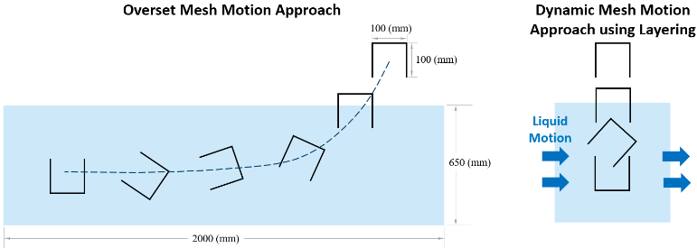
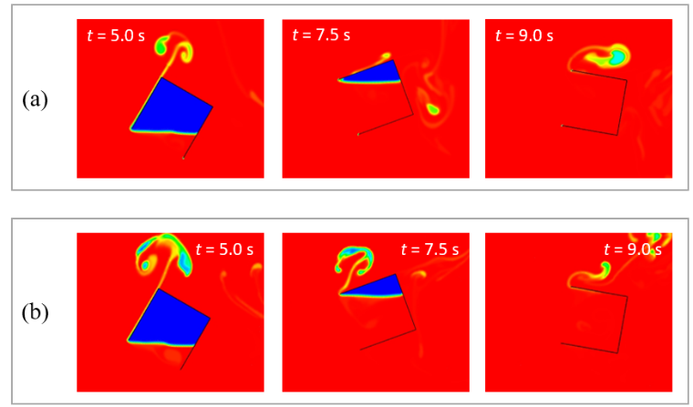
An inverted one-side open square box of edge length 100 (mm) is dipped into a water bath and rotated 180 deg along the motion path. Therefore, the air entrapped in the box when it is inside the water bath escapes gradually as the box is rotated. This square box can be considered representative of a cavity in the BIW that gets filled up during the e-dip process. Velocity magnitudes used in the motion profile are of the order of magnitude shown in Figure 4. Two cases are compared:

1. Overset mesh: It uses a “component” domain size of 150 (mm) x 150 (mm) around the box that moves over a fixed “background” domain of size 1 (m) x 2 (m). Overset method allows the overlayed component mesh to trace the actual motion path over the background mesh.
2. Dynamic mesh motion and layering technique: This applies the method proposed for e-dip simulations in this study. Therefore, domain decomposition is performed similar to that shown in Figure 5 (a).

Both the cases utilize the fluid properties listed in Table 1. Spatial discretization schemes are kept identical in both the cases while using PISO algorithm for pressure-velocity coupling. A fixed time-step size of 0.002 (s) utilizing the iterative time advancement method is employed in both the cases, with 15 iterations per time-step.

5. 2. Comparison of Results

Figure 8 compares the temporal evolution of the inner surface area of the box that is below the water level and still covered with air. Therefore, once the box starts dipping inside water and goes below the interface at around 2.1 (s), the surface area starts rising almost linearly. It starts to fall off once the box is rotated to allow the air to escape and water to fill in.

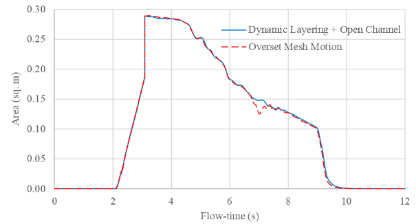
The instantaneous volume fraction plots are also compared in Figure 9. While the air escape patterns may differ between the two approaches due to absence of re-circulation path in the open channel-based approach, the capture of entrapped air inside the box compares very well. Overall, it is seen that the results are in very close agreement. Therefore, the proposed methodology can be considered to have captured all the relevant physics as against simulating the actual motion path.

6. Results and Discussion on the BIW e-dip

The four salient time points of the e-dip process are highlighted in Figure 10. Start of dip-in – t1: BIW just begins to touch the paint free surface; End of dip-in – t2: first instant when the BIW is completely dipped in; Start of dip-out – t3: BIW just touches the free surface again on its motion out of the tank; End of dip-out – t4: BIW is completely out of the tank.

During the e-dip motion, four quantities are specifically tracked:

1. Surface area of BIW covered with entrapped air below the paint level during the travel time t1 – t3
2. Volume of entrapped air during the same interval t1 – t3
3. Surface area of BIW covered with paint residue during the travel from t3 – t5
4. Volume of paint carryover during the same interval t3 – t5

Quantity (A) gives an estimate of area impacted by quality of deposition, while (B) gives an estimate of volume to be displaced to improve the process. Similarly, quantity (D) gives an estimate of the paint volume to be drained to avoid its carryover and contamination of downstream process tank. The resulting plots for these quantities are compared for iterative and hybrid-NITA solutions in Figure 10. It is seen that the predictions from hybrid-NITA nearly overlap those from the iterative solver.

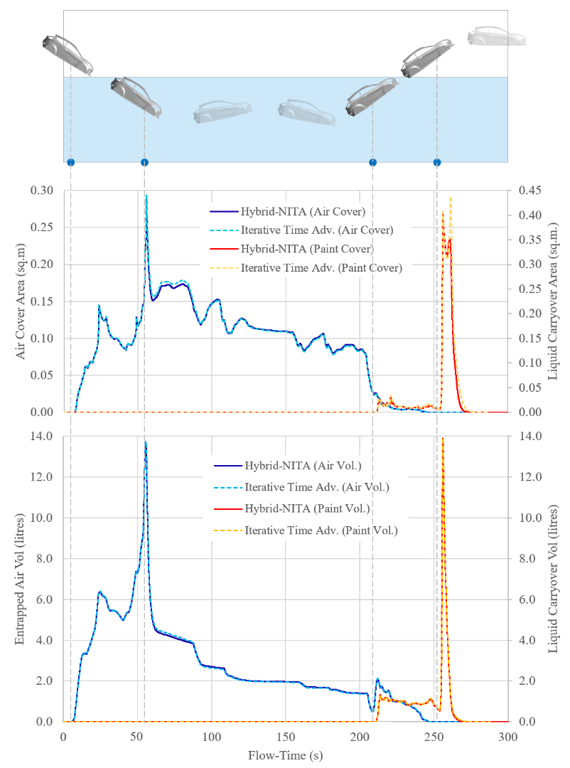
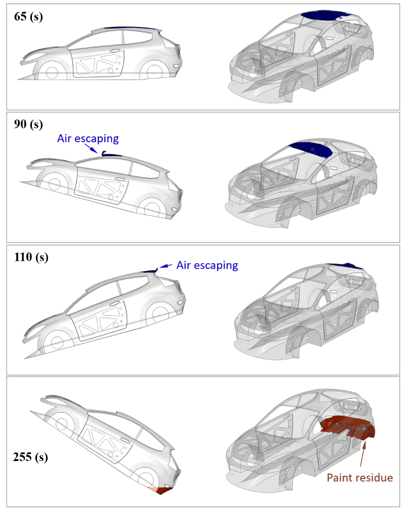
A spike of entrapped air is seen as soon as the dip-in is completed at t2. This results from the BIW rotating towards a horizontal position which entraps a large air pocket on the roof. Further, the two rocking motions between 80-120 (s) and between 150-190 (s) reveal an interesting trend. While the air volume entrapped drops during these periods almost monotonically, the surface area covered by entrapped air first drops during the forward tilt and then regains the original value on the way back to horizontal position. It then drops during the backward tilt and retains the drop, since the BIW geometry has a better escape path near the rear hatch compared to the front. This can be correlated to the images of entrapped air at t = 65, 90 and 110 (s) shown in Figure 11. This points to the fact that the volume entrapped, and surface area exposed to entrapped air may not be directly correlated and need to be looked at individually. It can be easily identified that the rocking motion aids in the partial removal of entrapped air pockets as compared to a straight travel. Similarly, during the dip-out, a spike in the liquid volume gets accounted around t4 when the dip-out is just completed and the rear-bottom of the BIW retains a considerable carryover liquid volume (refer Figure 11 at t = 255 (s)). However, it quickly drains out due to presence of holes on the rear and a very small residue of paint remains on the floor as the BIW turns back horizontal.

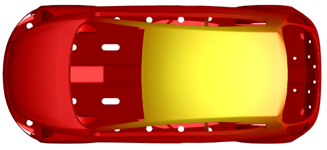
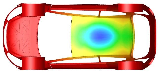
To evaluate the variation of paint contact time on various sections of the BIW, a user-defined variable was tracked during the travel from t2 – t3. During this time, a paint volume fraction weighted time was cumulatively stored for every surface element on the BIW. If the wall adjacent cell is filled with air, the contact time is considered as zero and if it is filled with paint, the contact time is accumulated based on paint volume fraction weighting function. Figure 12 shows the variation of contact time over the BIW at the end of dip-out. The trends of contact time clearly indicate that the inner surface of the roof panel has the least paint contact time due to the large, entrapped air bubble.

The results in Figure 10 are capturing the expected trends of bulk air entrapment and liquid drain volumes observed in typical production BIW models from OEMs. However, the accuracy of fluid volumes reported by simulations will be affected by the mesh resolution across the bleed holes and that in the proximity zones (like between BIW skins/surfaces on door panels). It is recommended to place at least one boundary element with 2-3 core cells to maintain a good numerical accuracy of volume fraction. Further, the "compressive" scheme used in Ansys Fluent ensures a bounded solution even for diffused volume fractions and avoids artificial numerical "oscillations" in the field. Finally, the mesh interface sliding between zones 2 and 3 should ensure the mesh motion Courant number maintained nearly equal to unity. This mesh Courant number will be a close function of horizontal motion velocity and cell sizes on the sliding interface and has been maintained as per this requirement in the present study.

7. Conclusion

In the present study, e-dip of an automotive BIW model was studied for two aspects (1) air entrapment in the paint bath and (2) liquid paint carryover after dip-out, using the VOF multiphase model in Ansys Fluent. Mesh motion considered in this study was decomposed into three components. Of these, two components of BIW dip-motion, namely, vertical translational motion and rotational motion were captured using a rigid body mesh motion, where the dynamic layering approach was used to accommodate the vertical motion. The horizontal component of BIW dip-motion was captured via the open-channel boundary setup available with the VOF model in Ansys Fluent. It was used to provide a continuous paint flow relative to the BIW motion. This methodology of capturing the dip-motion was first tested on a 2D model of a square cavity dipping into water. It was found to give results that were in very close agreement to those obtained from an overset mesh motion approach. This technique was then implemented on the representative BIW model of 4.7 million poly elements, using the iterative and Hybrid-NITA time advancement schemes. The simulations were run on a 96-core HPC cluster, with Intel® Xeon® Gold 6142 CPUs having a clock speed of 2.6 GHz. The Hybrid-NITA solver was found to give a 2.4X speed-up compared to the iterative solver, while giving similar accuracy of results. Thus, it can be concluded that the proposed mesh motion method along with the open-channel VOF setup and Hybrid-NITA scheme in Ansys Fluent provides a robust and fast technique to perform electro-dip predictions while using time-step sizes in the order of magnitude of 0.01 (s).

References

[1] N. Akafuah, S. Poozesh, A. Salaimeh, G. Patrick, K. Lawler, K. Saito, “Evolution of the Automotive Body Coating Process - A Review,” Coatings, 6(2), 24, 2016. View Article
[2] Z. Wicks Jr, F. Jones, S. Pappas, D. Wicks, Organic Coatings - Science and Technology (3rd ed.), John Wiley & Sons, 2006. View Article
[3] H.-J. Streitberger, K.-F.Dossel, Automotive Paints and Coatings (2nd ed.), John Wiley & Sons, 2008. View Article
[4] N. Akafuah, “Automotive Paint Spray Characterization and Visualization”, Automotive Painting Technology, Springer: Dordrecht, The Netherlands, 2013, pp. 121–165.
View Article[5] G. Zelder, C. Steinbeck-Behrens, “Simulation on Car Body Painting Processes,” 4th European Automotive Simulation Conference, EASC 2009, Munich, Germany, July 2009.
[6] A. Giampieri, J. Ling-Chin, Z. Ma, A. Smallbone, A.P. Roskilly, “A Review of the Current Automotive Manufacturing Practice from an Energy Perspective”, Applied Energy, vol. 261, 2020. View Article
[7] Ansys Fluent Theory and User’s Guide, Release 2021R1, Ansys Inc., 2021.