Journal of Fluid Flow, Heat and Mass Transfer (JFFHMT)

ISSN: 2368-6111

Nomenclature

1. Introduction

In recent years the market has indicated more demand to clean and sustainable alternative fuels, and natural gas has been regarded as a clean fuel with wide availability. Burning natural gas has shown a remarkable reduction in emission compounds, including carbon monoxide (CO), nitrogen oxides (NO_X), and particulate matter (PM). With a higher ratio of Hydrogen to carbon in natural gas properties compared to conventional fossil fuel such as gasoline and diesel fuel, the engine will produce even 20% less CO₂.

Shipping emissions are currently increasing, and due to the increase of global-scale trade, the trend gets even more in the future [1]. Moreover, the shipping industry's propulsion system plays a notable role in releasing hazardous emissions such as NO_X and SO_X [2,3]. LNG's utilization as the primary fuel of a lean-burn spark-ignition engine is one of the most promising solutions [4]. The lean-burn spark-ignition gas engine is Otto cycle theory working with an excess air ratio in the scale of lambda 2. This excess air reduces the engine components' thermal load during the combustion phenomenon and creates a steep decline in the NO _X compound [5]. In contrast to the lean combustion's earlier advantages, however, the emitted methane from the primary combustion due to incomplete combustion is considerable. This emission formation exposes a global warming potential 28 times higher than CO₂ in 100 years time scale [6].

In the marine propulsion system, the time-varying wakefield creates fluctuating engine loads, which may differ considerably from the time-invariant engine torque estimated in steady conditions. Providing a stable operational condition gets even worse when the engine torques and the thermal load are low. Supplementary control of the airflow by an air throttle to restrict the extra air improves the flame quality. This additional control is performed in the pioneer manufacturers as well [7].

The effect of intake throttling has been studied predominantly on the CI and SI engines [8,9]. The intake-throttling device enhanced EGR injection by reducing the pressure behind the intake valve, and it effectively accelerated the natural gas combustion [10]. In contrast, due to the pumping losses caused by partially opened of the throttle in the air passage, the engine's efficiency decreased during lower loads. Therefore, using early intake valve closure (EIVC) on intake valves was proposed to improve the combustion quality in direct injection gasoline engines. Ojapah et al. [11] developed this idea by testing a single-cylinder engine and concluded that EIVC contributed to combustion efficiency improvement. The drawback was increasing the UHC formation due to slower combustion compared with throttle control. In addition to the requirements to examine the effect of the air throttle on engine response, the mechanical delay or the turbocharger lag is a notable off-design feature of the turbocharged engines during the transient condition. This feature distinguishes the response of the engine in transient condition with the steady-state. If all the differences are classified in thermal delay, mechanical delay, and dynamic dealy, part of the mechanical delay is associated with the turbocharger lag. It is agreed that when the engine is under transient operation, the energy transported by the exhaust gases arrives very quickly at the turbine [12], even with the fastest feedback caused by the fuel system to compensate for the deviation of the torque or demanded speed, the compressor air-supply cannot match this higher fuel-flow instantly [13]. For the lean-burn gas engine, this lag led the mixture to a lower value during load increment and a higher value during load decrement [14]. Since the combustion of the lean-burn spark-ignition engines is critically sensitive to the air excess ratio, this phenomenon reduces the combustion efficiency and increases the NO_X.

This study evaluated the air throttle influence during lower loads in steady-state and transient conditions by returning to the hypothesis posed in this section. Moreover, the turbocharger lag is also modeled and discussed throughout a marine time-varying load. Thus, a thermodynamic engine model was developed to model a marine gas engine. The engine was simulated with an imposed constant torque for the steady-state condition, and two imposed changeable torques for the transient state. In the next sections, the modeling procedure is first presented in Section 2, and the primary output is verified with the engine measured data. The imposed loads are presented in Section 3, and the throttle assessment in lower loads plus the turbocharger lag is discussed in Section 4. The conclusion is expressed in Section 5.

2. Simulation Method

2.1. Implemented Equations

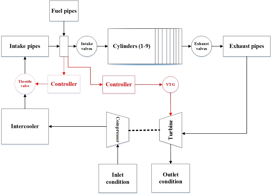
A thermodynamic model was performed by GT-suite 2019 software. This program simulated the dynamic of the inlet and outlet gases, turbocharger performance, and combustion flame characteristics. Depending on the model's type, the simulation could be predictable, semi-predictable, or non-predictable [15]. The thermodynamic process model commenced from the atmosphere with a boundary inlet temperature and sea level pressure. It was continued to the compressor with an implemented performance map or look-up table from the manufacturer. The converted thermodynamic energy from the turbocharger mechanical shaft provided a high boost pressure and the inlet air temperature. A charge air cooler received the high-temperature air at the entry, and it delivered the low temperature air with some pressure drop. In order to simulate the dynamics of the airflow in the pipes, the equations of momentum were derived together with energy and mass conservation in the discretized volume. To estimate the mass flow rate over the intake and exhaust valves, a one-dimensional isotropic flow analysis for compressible flow through a flow restriction was performed [16].

Combustion was modeled in all the cylinders by implementing the flame propagation model [17], and the emission formation was calculated using the proposed reaction rates for the species estimated in the equilibrium for the essential species, such as N₂, O₂, CO₂ . Afterward, the burned gas was passed via the exhaust valves and exhaust ports. The high enthalpy gas of the exhaust carries considerable thermal energy, and it drives the turbine to generate torque to rotate the connecting shaft and compressor. Then, the low enthalpy gas discharges into the atmosphere, and the cycle becomes complete. The specification of the marine engine is presented in Table 1.

Table 1: Engine specification

Item	unit	amount
Number of cylinders	-	9
Cylinder bore	mm	350
Cylinder stroke	mm	400
Connecting rod	mm	810
Maximum power	kW	3940
Rated speed	rpm	750
Maximum Torque at rated speed	Nm	50200
Fuel type	-	Natural gas

A detail of the implemented equations was presented in work by these authors in [18]. The available measured data, such as sea boundary condition, wall temperatures, spark plug locations, and timings were all imposed in the simulation model. A schematic of the engine modeling and the air throttle position is shown in Fig. 1. Due to the importance of the flow modeling in predicting the dynamic and mechanical delay of the engine response, these two items are developed in this section. Further modeling can be found in [19].

To calculate the dynamic delay of the fluid flow and consequently the turbocharger response, the equations of conservation are involved the conservation of momentum as well as Equation (1) and (2) [20].

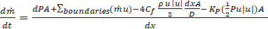
Where m is mass of volume, and m^. is the boundary mass flux. A is the cross-sectional flow area, and A_S is the heat transfer surface area.

In the discretized volume, the Equation (1) and (2) yield the mass and energy in each volume. With the available volume and mass, the density can be calculated. Afterward, the equations of state define density and energy as a function of pressure and temperature, and the solution will be continued iteratively on pressure and temperature until they satisfy the density and energy already calculated for this time step.

A turbocharger consists of three components: The turbine, the compressor, and the connecting shaft. These components have a mass moment of inertia, which is influential in the turbocharger rotational speed. The higher the moment of inertia, the more time to reach the new stable speed. The rotational speed is a function of pressure ratio, efficiency, and flow rate of compressor and turbine. Thus, a performance map from the manufacturer is imposed on the modeling. Turbocharger speed and pressure ratio are predicted at each time-step, and two other unknowns are taken from the look-up table [21].

The calculation starts with Equation (4) and predicted pressure ratio and calculating total temperature by Equation (5).

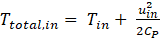
where u_in is inlet velocity. The outlet enthalpy will be calculated by Equation (6) and the compressor power by Equation (7) provide subsequently the torque of the compressor.

where subtext script in, out and s stands for inlet, outlet and isotropic, respectively. Using equations (8), the new calculated rotational speed is provided.

For the turbine, the following equations are employed:

The computation will be repeated until the predicted parameters reach an acceptable convergence.

2.2. Validation

The model is validated both in steady-state and in transient conditions. Comparing experimental and simulation output verifies that the model could accurately predict the engine performance and emission compounds. Table 2 presents the validation for a steady-state. Normalized BSFC for performance prediction and normalized UHC for emission prediction is given. As can be seen, there is always a negligible difference between the modeling and the measured data. In the worst case, the deviation for UHC in 75% load is 8.3%, and it is still acceptable.

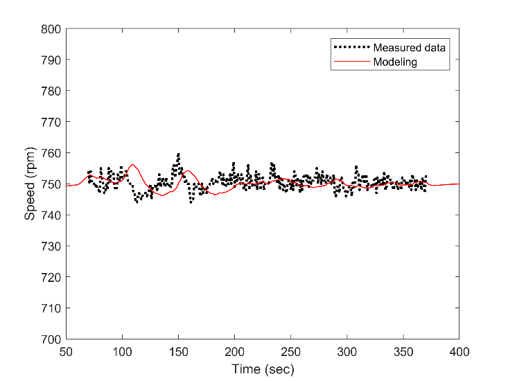
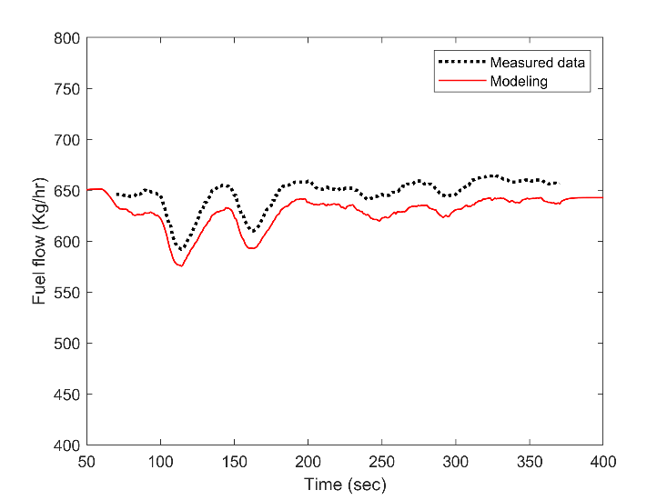
Furthermore, Fig. 2 shows that during the in almost 300 seconds of the load variation of the transient condition, the operating engine tried to maintain on 750 rpm, and the modeling is also showing the same trend with a minor difference. Fig. 3 presented the fuel flow rate. This figure displays an acceptable agreement of the simulation results with the time-varying load. There is a difference between the modeled flow rate and the operational value, but this deviation is almost constant during the time. The main reason for this difference could be the difference in modeling the friction of the components, such as friction in the cylinders as fmep. This friction was assumed to be constant during the time-varying load in the engine modeling.

Table 2: Engine model verification during the steady-state with a comparison of measured and simulated data.

Load (%)	Torque (Nm)	BSFC (Normalized)			UHC (Normalized)
		Measured	Theory	Deviation(%)	Measured	Theory	Deviation(%)
100	50200	1	1	0	1	1	0
85	42670	1.029	1.018	1	1.11	1.05	5.4
75	37650	1.045	1.034	1	1.20	1.10	8.3
50	25100	1.089	1.108	-1.7	1.37	1.30	5.1
25	12500	1.374	1.334	2.9	2.0	2.01	0.5

3. Implemented Steady and Transient Torque

In order to evaluate the significance of throttle in the lower loads of a lean-burn spark-ignition gas engine, two operating loads were studied, steady-state and unsteady state.

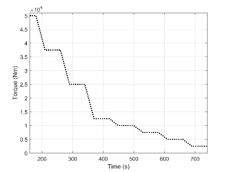
For the steady-state condition, the implemented load reduced from 100% to 50%, 25%, 20%, 15%, 10% and 5%. 100% and 50% mean 50000 and 25000 Nm, and the airflow is regulated with the standard variable turbine geometry (VTG) controller. In the 25% load and less, which are 12500 Nm and less, the throttle also regulated the amount of airflow. The throttle controller consisted of a conventional PID controller with two sensors from air and fuel pipes to calculate the ratio and one actuator to change the throttle valve degree between 0 to 90. The load-time curve for steady-state is shown in Fig. 4.

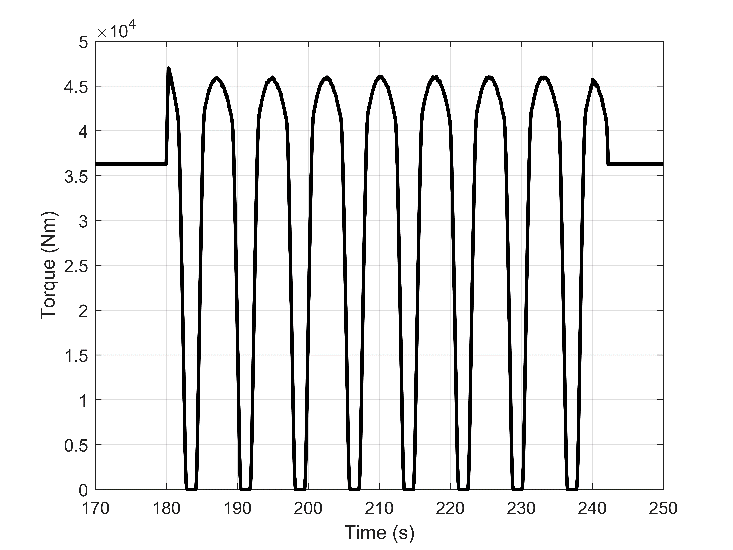
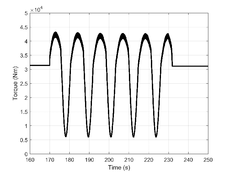
An identical controlling pattern of VTG and throttle was utilized for the transient condition. The estimated harmonic load against harsh weather conditions is shown in Fig. 5. A ship traveling in various wavelengths, wave amplitudes, and wave directions influences the wave size and changes the thrust and torque fluctuations. More detail of the wave calculation is presented in [22]. This wave amplitude and frequency satisfied our requirement for modeling the marine engine in a broad spectrum of loading. The brake torque changed from a constant value of 36000 Nm in the second 180 to almost 45000 Nm and then reduced to zero. The wave period was nearly seven seconds, which has around four seconds for the higher loads, and fewer than three seconds for the loads less than 30%, the duration when the throttle is active.

In addition, another wave characteristic was considered for the turbocharger lag assessment. This wave has a lower frequency and amplitude; then, it is more understandable to recognize the mechanical lag caused by the turbocharger. The implemented wave is shown in Fig. 6.

4. Results and Discussion

The nominal engine speed of 750 rpm was chosen for the modeling. The engine speed operated around the constant value by adjusting the fuel rack position with a PID controller. The result section is divided into two parts. First, the impact of the ait throttle is discussed during the steady-state and transient conditions. Afterward, the turbocharger lag is presented by considering several inputs to the mass moment of inertia. The inertia's base value is considered one, and the others are relative values with the coefficients of 0.5, 0.75, 1.25, 1.5, and 2.

4.1. Throttle Assessment

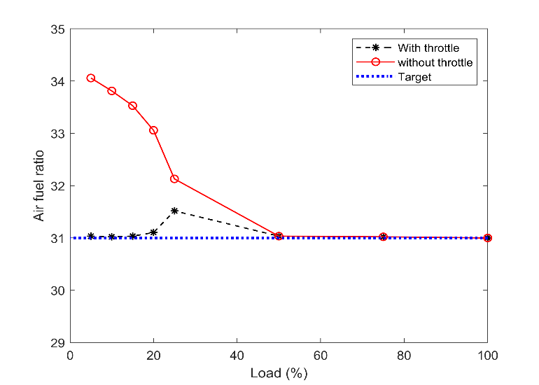
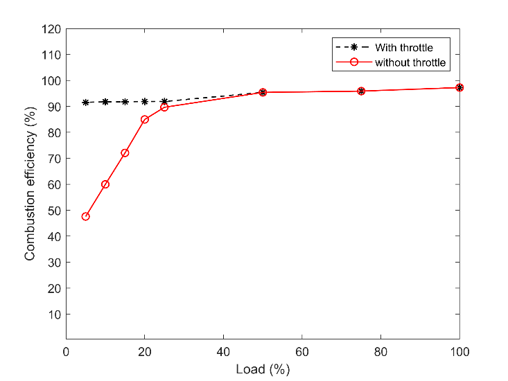
Fig. 7 illustrates the air-fuel ratio comparison in a steady-state with and without throttle. A target setpoint, which is a constant quantity of 31, was also shown. As can be seen, during steady-state with a throttle, the air-fuel ratio stayed equal to the setpoint. However, there was an exception with the 25% load. This deviation may stem from numerical error and is negligible. While without the throttle, the ratio grew up to 34 during lower loads. This ratio is extremely lean for stable combustion, and it results in quenching the flame. Fig. 8 shows that the combustion efficiency reduces during the lower load if there was no throttle on the air passage. Besides, with the throttle, combustion efficiency lingered almost constant with load change since the air-fuel ratio was consistent.

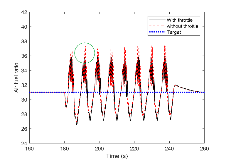
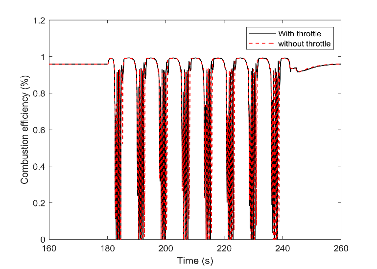
In contrast, Fig. 9 shows that using a throttle during the transient load was not adequate for regulating the amount of air. This is indicated in the figure using a circle. Therefore, the excess ratio always exceeded the setpoint with or without throttle. The combustion efficiency also shows the same pattern, as shown in Fig. 10. Referring to the frequency of the waves in Fig. 5 and based on the results, we can conclude that this small time scale is extremely short for the throttle to turn into convergence. Therefore, for such high-frequency waves, a device with a more rapid response is needed to provide acceptable stability.

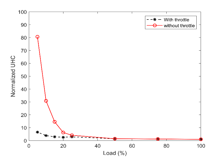
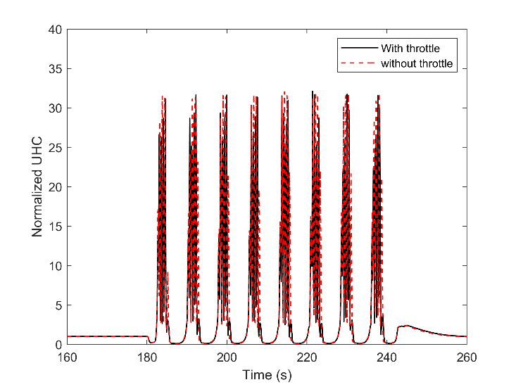
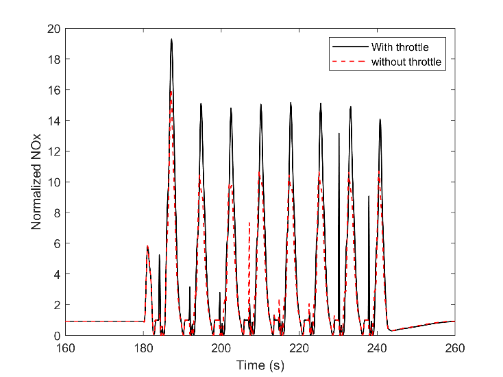
The data obtained for the emission formation, NO_X and UHC, are broadly consistent with the performance output's major trends. Fig. 11 and Fig. 12 displayed the variation of unburned hydrocarbon in these two operational modes, with and without throttle. These authors' previous work [14] revealed that the UHC compound directly correlates with the air-fuel ratio, and a higher amount of excess air ratio deteriorated the combustion quality and resulted in the flame quench. Besides, flame quench was one of the three primary UHC sources in lean-burn spark-ignition gas engines together with gas exchange and crevice volume. Therefore, a significant part of the fuel remained unburned when the excess ratio increased to a value more than the setpoint. When the load declines, the fraction of unburned fuel will increase as well. As shown in Table 2, the measure data proved that the UHC quantity in 25% load is doubled compared with 100% load. Following the same trend in Fig. 11 shows seven times UHC increases with a 5% load when the engine is working in steady-state and with the throttle. Skipping the throttle may increase the UHC up to 80 times higher value. This amount of unburned fuel results in almost twice fuel consumption during the lower loads. Hence, the significance of using a throttle during lower loads can be proved in the emission aspect as well, even though it is not beneficial in transient conditions, as shown in Fig. 12.

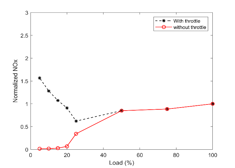
Furthermore, NO_X showed a contrast procedure compared with the UHC compound, as shown in Fig. 13 and Fig. 14. This emission compound is deeply relevant to the flame temperature [16]. With a higher air-fuel ratio, the combustion chamber's thermal load declined, and the amount of NO_X was reduced. It worth mentioning that in Fig. 13, there is a sudden reduction for the 25% load for the engine output with a throttle. Part of this reduction of NO_X stems from the unexpected higher air-fuel ratio, as was mentioned in Fig. 7.

4.2. Turbocharger Inertia

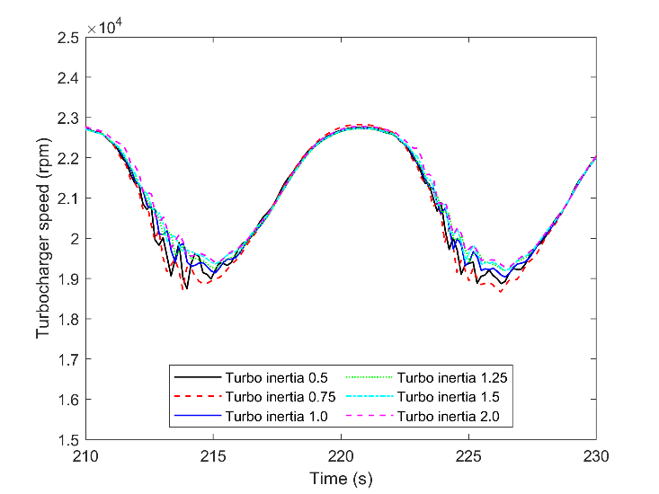
The previous section about transient engine operation clearly showed the engine mechanical and dynamic delay with the corresponding variation in implemented torque during the transient times. The modeled engine that is the object of this study has input inertia equal to the manufacturer's value. A different value for the inertia is assumed to predict a more accurate evaluation of the turbocharger lag. Both the increment and decrements of the inertia influence the lag of the turbocharger by changing turbocharger speed. The turbocharger rotational speed is shown in Fig. 15.

For clear visibility, part of the wave is presented. During the load variation, the shaft rotational speed varies between 19000 to 23000. This domain is almost constant for all of the inertia. It shows that the other components dynamic and the magnitude of the waves are crucial governors on engine performance when the engine response is on an investigation. However, in a short time scale, the small scale variation occurs when the load decreases. The inertia, with a coefficient of 0.5, has the most considerable oscillation. During the load increment, all of the cases have a smooth response to the load.

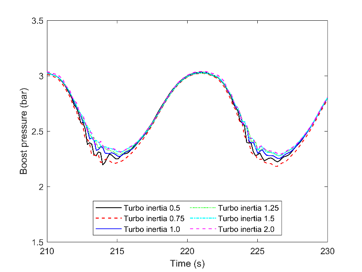
The turbocharger with a coefficient of 2.0 has the least oscillation, but the turbo speed is the highest throughout the time. This means that the total speed reduction for the high inertia is the lowest. Almost the same approach is obtainable for the boost pressure in Fig. 16. During the load increment, all the cases have the same boost pressure, while during the load reduction, more drop and more fluctuation is achieved by low shaft inertia. Moreover, this figure confirms that the available turbocharger shaft inertia, coefficient 1, is chosen correctly. The blue line has the minimum difference with higher inertia but a noticeable distance to the lower inertia. This proves that increasing the shaft inertia will not contribute to a remarkable enhancement of boost pressure.

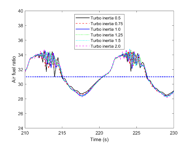
The oscillation of the turbocharger and its influence on the air-fuel ratio is visible in Fig. 17. The air-fuel ratio is continually reducing during load increment, and there is a negligible difference between the cases. However, the response is different during lower loads, in this figure for the seconds between 210-216 and 222 to 226. The turbocharger inertia with a coefficient of 0.5 with the black line gives a huge oscillation in the time scale of seconds. With an engine speed of 750 rpm, the different air-fuel ratios in different subsequent cycles are possible. It can be more noticeable if the intake manifold and the fluid dynamic do not distribute the flow equally. As a consequence, there would be lots of variation between the cycles and the cylinders.

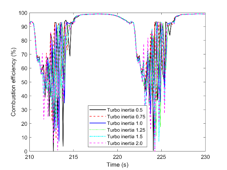
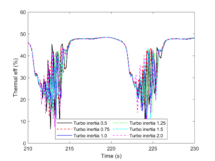
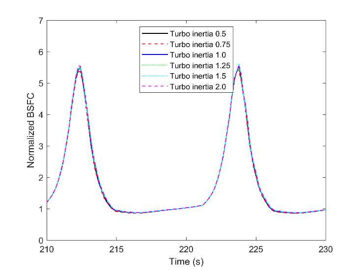
Considering the combustion efficiency in Fig. 18, as the fraction of the burned fuel to the total injected fuel, and thermal efficiency in Fig. 19, as the fraction of brake work to the total injected energy, there are striking variations. With increasing the turbocharger lag, the variation reduces, and the engine moves toward more stable combustion. This output clears how vital is the turbocharger performance on combustion efficiency, thermal efficiency, and stability of the engine during the transient marine condition. However, the total fuel consumption and the fuel flow average are almost constant for all cases. BSFC is shown in Fig. 20, and it is hardly possible to figure out the differences between the simulation cases. The noticeable output from this figure is the variation of the BSFC during the marine wave, where it increased from a normalized value of one to more than 5. The BSFC of the times before 170, as steady-state, was chosen for normalizing.

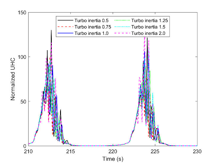
The same normalizing value was chosen for NO_X and methane slip, UHC. The UHC is defined as the unburned fuel of the combustion chamber, which has not participated in the main combustion and post-oxidation. It is used to evaluate how well a gas engine converts the natural gas to work and heat. This compound is a function of fuel-burning rate and main chamber temperature. When the air excess ratio increases, the burning rate of natural gas reduces, and the maximum temperature decreases: the extra air leads more lean mixture and further temperature reduction. Consequently, lots of the fuel will not burn during the main combustion process, and since the temperature during post oxidation is low, a striking increase of the methane slip is achievable. Comparing the air-fuel ratio in Fig. 17 and Fig. 21 confirms how influential is the air excess ratio. UHC increase to 100 means 100 times more quantity than the nominal value in steady-state. This is one of the main reasons for BSFC increase during lower loads. If this additional fuel is trapped in the chamber or be controlled before the load reduction, fuel consumption reduces significantly.

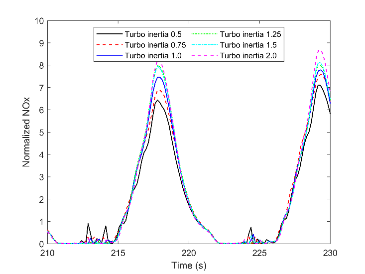
In contrast with the UHC, even though the higher inertia improved the engine combustion during load reduction, the engine's lag during load rise resulted in a richer mixture and extra maximum temperature. The higher temperature forms a more quantity of NO _X , and for this reason, there is more NO _X with the highest shaft inertia during load increment, the time between 216 to 222. Moreover, similar to the other figures, the long time scale variation of NO_X is in the same frequency as the other figures, and it changes from almost 0 in low loads to 7 in high loads. The trend is shown in Fig. 22.

5. Conclusion

This work emphasized the engine performance, i.e., the dynamic response, combustion efficiency, and emission resulting from the constant load and oscillating propeller load. There was a particular interest in examining the throttle adjustment and turbocharger lag on the engine response. A thermodynamic spark-ignition engine model was developed, and based on the findings presented in this paper; the results can be summarized as:

• The engine was effectively regulated with the throttle during lower loads of the steady-state. The throttle exceptionally determines the fuel consumption and the emission formation and uninstalling the throttle valve results in incomplete combustion and lots of unburned hydrocarbons.
• For the transient condition when the frequency is high, the throttle did not recover the engine characteristics during lower loads. It was shown that the time scale of the throttle angle for the newly adjusted setpoint was longer than the waves' period.
• The created delay in providing the new throttle angle restricted a rapid response by the engine, especially in harsh weather conditions. Therefore, the application of the throttle valve in the fast-transient state is worthless.
• The mass moment of inertia directly influences the turbocharger speed and, consequently, boosts pressure and airflow.
• The lower the mass moment of inertia, the less stability on the turbocharger. This led the engine to fluctuate significantly due to variation in air excess ratio.
• A very high mass moment of inertia may improve the engine response when the load drops, but during load increment, the more lag resulted in higher NO_X formation due to increased response time.

References

[1] M. Viana, P. Hammingh, A. Colette, X. Querol, B. Degraeuwe, I. de Vlieger, andJ. van Aardenne, “Impact of maritime transport emissions on coastal air qualityin europe,”Atmospheric Environment, vol. 90, pp. 96 – 105, 2014. View Article
[2] E. Fridell, E. Steen, and K. Peterson, “Primary particles in ship emissions,”At-mospheric Environment, vol. 42, no. 6, pp. 1160 – 1168, 2008. View Article
[3] V. Matthias, I. Bewersdorff, A. Aulinger, and M. Quante, “The contribution ofship emissions to air pollution in the north sea regions,”Environmental Pollution,vol. 158, no. 6, pp. 2241 – 2250, 2010. Advances of air pollution science: fromforest decline to multiple-stress effects on forest ecosystem services. View Article
[4] S. Ushakov, D. Stenersen, and P. M. Einang, “Methane slip from gas fuelledships: a comprehensive summary based on measurement data,”Journal of MarineScience and Technology, vol. 24, no. 4, pp. 1308–1325, 2019. View Article
[5] D. Stenersen and O. Thonstad, “Ghg and nox emissions from gas fuelled engines:Mapping, verification, reduction technologies,” Tech. Rep. OC2017 F-108, SIN-TEF Ocean AS, NO-7465 Trondheim NORWAY, 2017.
[6] T. I. P. on Climate Change, “Global warming potential values,” 2016. IPCC FifthAssessment Report.
[7] “Project guide: Bergen engine type b, fuel gas operation,” tech. rep., BergenEngines AS, 2018.
[8] J. Reß, C. St ̈urzebecher, C. Bohn, F. M ̈arzke, and R. Frase, “A diesel engine modelincluding exhaust flap, intake throttle, lp-egr and vgt. part i: System modeling,”IFAC-PapersOnLine, vol. 48, no. 15, pp. 52 – 59, 2015. 4th IFAC Workshop onEngine and Powertrain Control, Simulation and Modeling E-COSM 2015. View Article
[9] V. B. Pedrozo, I. May, T. D. Lanzanova, and H. Zhao, “Potential of internal egrand throttled operation for low load extension of ethanol–diesel dual-fuel reac-tivity controlled compression ignition combustion on a heavy-duty engine,”Fuel,vol. 179, pp. 391 – 405, 2016. View Article
[10] J. You, Z. Liu, Z. Wang, D. Wang, Y. Xu, G. Du, and X. Fu, “The exhausted gasrecirculation improved brake thermal efficiency and combustion characteristicsunder different intake throttling conditions of a diesel/natural gas dual fuel engineat low loads,”Fuel, vol. 266, p. 117035, 2020. View Article
[11] M. Ojapah, Y. Zhang, and H. Zhao, “Part-load performance and emissions analy-sis of si combustion with eivc and throttled operation and cai combustion,” inIn-ternal Combustion Engines: Performance, Fuel Economy and Emissions, pp. 19– 32, Woodhead Publishing, 2013. View Article
[12] N. Watson and M. S. Janota,Introduction to Turbocharging and Turbochargers,pp. 1–18. London: Macmillan Education UK, 1982. View Article
[13] C. Rakopoulos, A. Dimaratos, E. Giakoumis, and D. Rakopoulos, “Evaluation ofthe effect of engine, load and turbocharger parameters on transient emissions ofdiesel engine,”Energy Conversion and Management, vol. 50, no. 9, pp. 2381 –2393, 2009. View Article
[14] S. Tavakoli, M. V. Jensen, E. Pedersen, and J. Schramm, “Unburned hydrocarbonformation in a natural gas engine under sea wave load conditions,”Journal ofMarine Science and Technology, 2020. View Article
[15] GT-SUITE, “Flow theory manual,” tech. rep., Gamma Technologies, 2017.
[16] J. B.Heywood,Internal Combustion Engines Fundemental. New York: McGraw-Hill, Inc, 1988.
[17] N. C. Blizard and J. C. Keck, “Experimental and theoretical investigation of tur-bulent burning model for internal combustion engine,”SAE, p. 740191, 1974. View Article
[18] S. Tavakoli, E. Pedersen, and J. Schramm, “Natural gas engine thermodynamicmodeling concerning offshore dynamic condition,”Proceedings of the 14th Inter-national Symposium, PRADS 2019, September 22-26, 2019, Yokohama, Japan,vol. II, 2019.
[19] S. Tavakoli, S. Saettone, S. Steen, P. Andersen, J. Schramm, and E. Pedersen,“Modeling and analysis of performance and emissions of marine lean-burn natu-ral gas engine propulsion in waves,”Applied Energy, vol. 279, p. 115904, 2020. View Article
[20] GT-SUITE, “Engine performance,” tech. rep., Gamma Technology, 2017.
[21] A. Sidorow and R. Isermann, “Physical and experimental modeling of turbocharg-ers with thermodynamic approach for calculation of virtual sensors,” (Rueil-Malmaison, France), 2012. View Article
[22] S. Saettonea, B. Taskara, P. B. Regenera, S. Steen, and P. Andersena, “A compar-ison between fully-unsteady and quasi-steady approach for the prediction of thepropeller performance in waves,”Applied Ocean Research, vol. 97, 2019 View Article