Journal of Fluid Flow, Heat and Mass Transfer (JFFHMT)

ISSN: 2368-6111

1. Introduction

Despite international efforts to restrict fossil fuel production, the trend in emissions is still upwards [1]. Fossil fuels continue to dominate the electricity and wider energy mix in many regions of the world and are expected to do so for the next decades [2].

In 2015 at the 21^st Conference of Parties (COP21), all the participating nations undertook major steps to mitigate climate change and limit global temperature increases to “well below 2 oC” compared to pre-industrial levels [3]. The countries agreed that climate change mitigation would account for more than 80% of global GHG emissions. To stall the temperature increase below the threshold of 2 oC a limit has been set on the amount of CO₂ to be emitted by 2100, referred as a “global carbon budget” [4], which is 1170 Gt CO₂; for a 1.5 oC limit the budget is only 420 Gt. The IPCC has identified certain measures, essential to enable us to stay within the available carbon budget, which include among others, increases in energy efficiency, employment of renewable energy sources in the power sector, carbon capture and storage technologies, and reduced dependency on fossil fuels [5], [6].

The aim of this study is to employ Hubbert’s logistic function to estimate the future unconstrained production of fossil fuels across different regions of the world. This projection is only feasible and accurate if the historical data are fitted adequately. After estimating the production projections and applying the essential emission factors for natural gas, oil and coal, the calculation of CO₂ emissions is possible. In this way, we are able to understand what share of the available budget is consumed, and to test if the trend in production is compatible with preventing dangerous climate change.

2. Methodology

Hubbert’s logistic function, was used originally to match oilfield production [7]. The same function is used for many other purposes, such as to model population growth and in epidemiology. In this study, it is used to fit past data of fossil fuel production (natural gas, oil and coal). Cumulative production is given by:

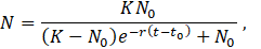
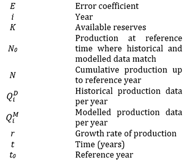
where N is the estimated production, K refers to the proven reserves while N₀ is calculated so that modelled production at reference time, t₀ which is set to be 2018, matches the historical data value Q^D. The unconstrained growth rate of production is represented by r.

The first derivative of Eq. (1), which represents the rate of production, produces a bell-shaped curve:

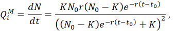
where, is the modelled production rate.

The factors affecting the shape of the curve, are K and r and are defined by:

The above equation is solved using Eq. (2) to find N₀ for . The fitting error in such methodology must be examined, as in some cases a good fit is not possible for reasons explained in the next section.

For the calculation of emissions, conversion factors for oil, natural gas and coal available in the literature were used to convert fossil fuel production measured in energy equivalent to CO₂ emissions [8]. The conversion factors applied are the following:

NG:     56100  / 23.8 × 1000 = 2.35

COAL:            93100  / 23.8 × 1000 = 3.91

OIL:  74100    / 23.8 × 1000 = 3.11

Fossil fuels in the extraction industry are traditionally measured in a mixture of units: billion cubic meters for natural gas, mega-tonnes for coal, and billion barrels for oil. Such units are transformed to mega-tonnes of oil equivalent (Mtoe) of primary energy to calculate the associated CO₂ emissions according to the following transformations:

            NG:                 bcm    ->        Mtoe  ×         0.86

            COAL:            Mt       ->        Mtoe  ×         0.58

            OIL:               bb       ->        Mtoe  ×         0.90

For the production projections, only current technologies available are taken into account, as the model does not account for technological developments; for instance, the original Hubbert model could not predict the recent rise in US oil production from shale. In addition, no economic or political variables are taken into consideration, assumptions that in some cases cause the deviation of curves from historical data. The initial data for current recoverable reserves considered are obtained from the BP statistical review of world energy 2019 [9].

3. Results and Discussion

SThe Hubbert curves were determined for seven world regions: North America (NA), South, Central America (SCA), Europe (EU), Middle East (ME), Asia & Pacific (AP), Africa (AFR) and Commonwealth of Independent States (CIS), and for the three principal fossil fuels, oil, gas and coal. Using Eq. (1) we are able to determine the cumulative production considering the available data on growth rate and available reserves; to create the bell-shaped Hubbert’s curve, we need its first derivative that is given by Eq. (2)

Error Analysis

In this study, an error analysis was conducted to determine which curves adequately fit the historical data. To determine the quality of the data match, the following correlation coefficient is used:

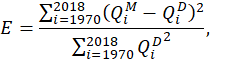
where i labels the year from 1970 to 2018 where there are available data. The E value calculates the deviation of predicted values from historical data. Q_i^D and Q_i^Mrefer to the historical and predicted data respectively, while K, r are determined with a try and error method, that returns the minimum value of E.

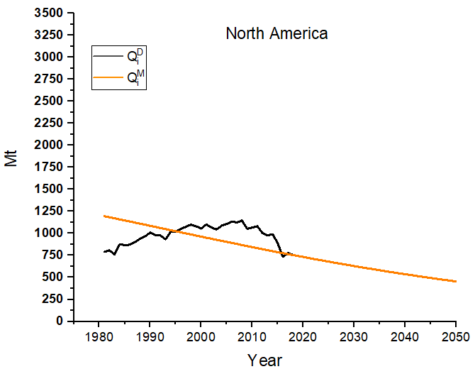
E, was determined for oil, natural gas and coal production and reported in tables 1, 2, and 3 respectively. If E was greater than 10%, the regions were excluded from the study. North America was excluded from coal study and Europe, CIS and Africa from the oil one, while natural gas curves fitted adequately all the regions considered.

Oil Production

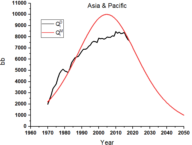
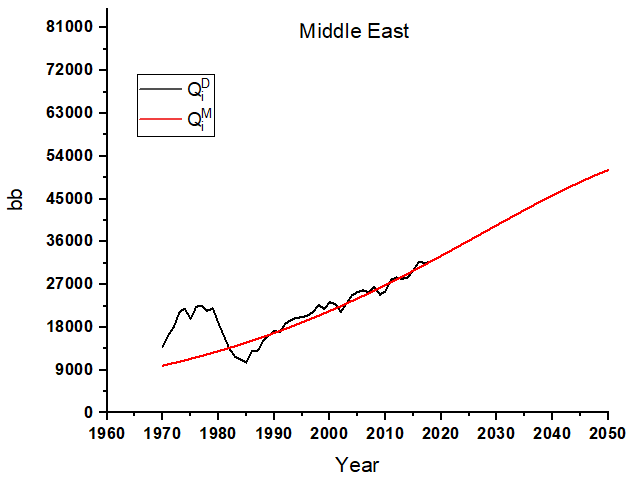
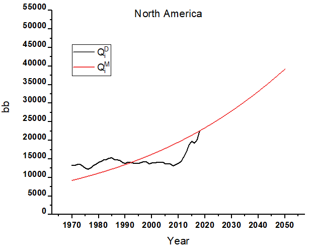
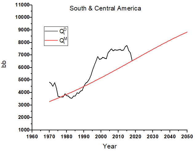
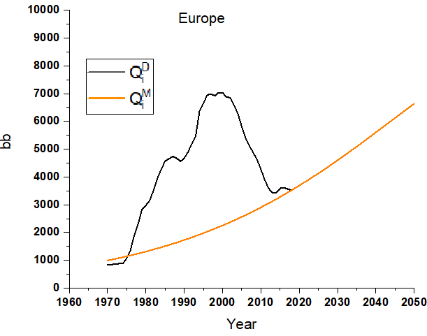
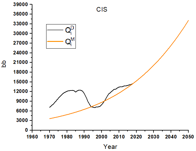
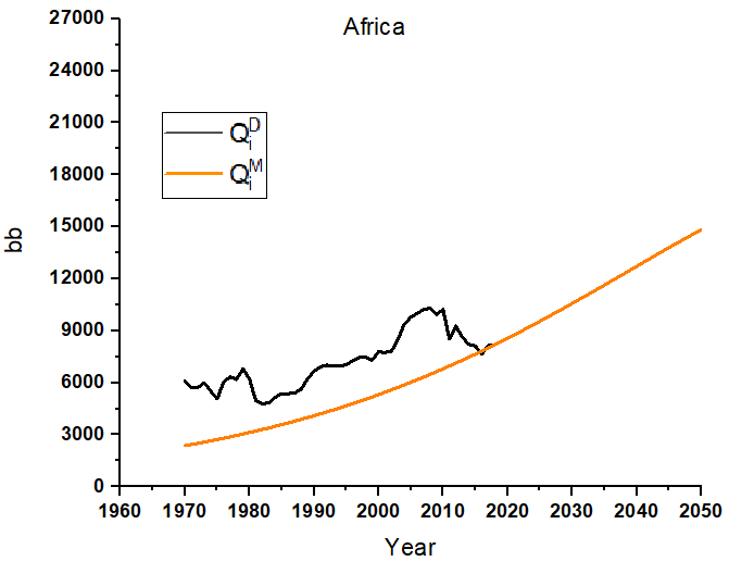
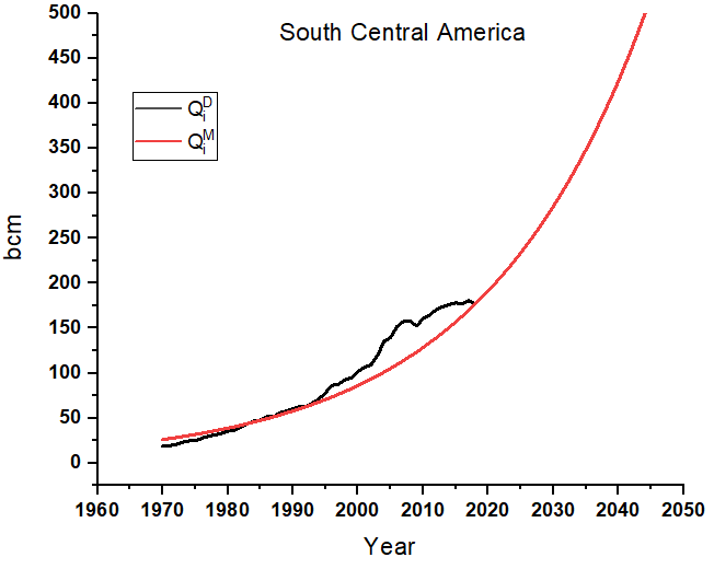
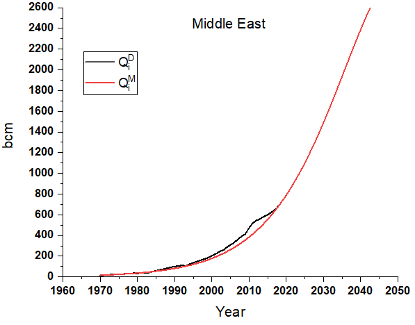
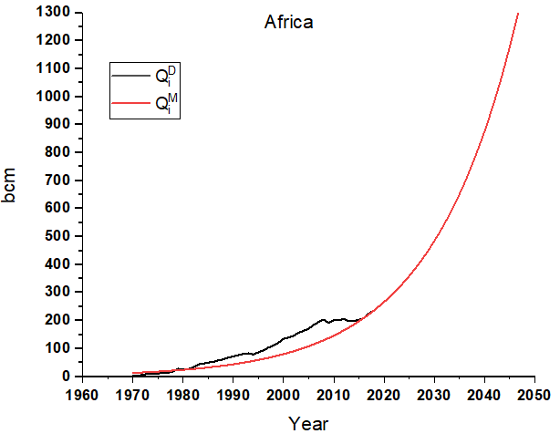
Major oil producing regions, such as the Middle East and North America, are projected to continue oil production for several years as they possess vast reserves as can be seen in Figure 1. For the AP regions, the logistic function projects that peak production occurs around, 2015. According to Table 1, Africa, EU and CIS present a match with E value to be greater than 10% and are therefore excluded from the study (Figure 2).

Table 1. Error in the regions for oil production.

Region	E (%)
Asia & Pacific	3.13
South, Central America	3.55
Middle East	3.84
North America	4.26
Africa	12.7
CIS	13.8
Europe	36.4

Natural Gas Production

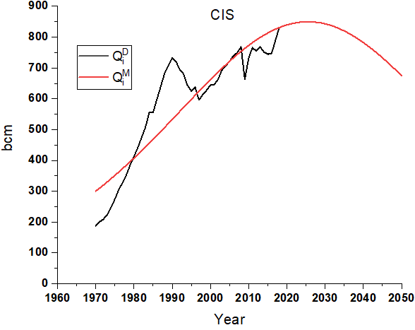
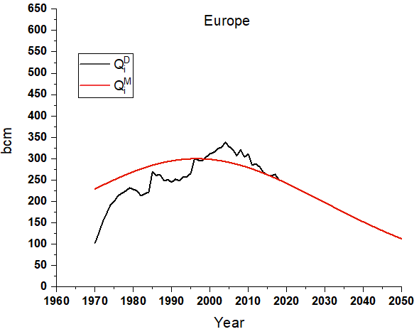
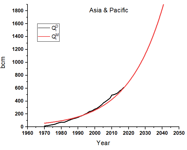
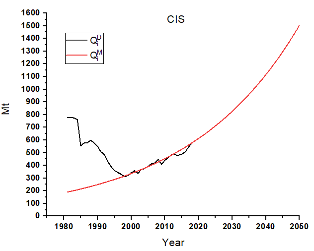
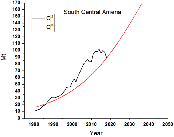
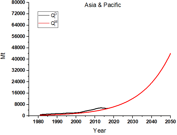
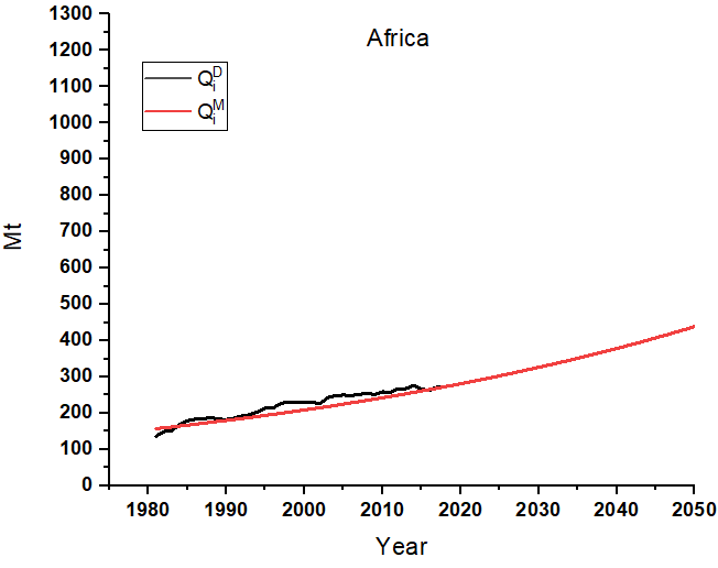
For natural gas production, according to Table 2. the Hubbert model fits the data well for all the designated regions of the study. Figure 3, demonstrates how production is expected to increase in all the regions considered, while in the CIS and Europe regions, a peak seems to have been reached already.

Table 2. Error in regions for natural gas production.

Region	E (%)
Asia & Pacific	0.85
Middle East	1.55
CIS	1.74
North America	1.96
Europe	2.76
South, Central America	2.92
Africa	7.55

Coal production

For coal production four regions can be accurately fitted to Hubbert curves as observed in Figure 4. According to Table 3. North America presents a poor fit and therefore is excluded. To the rest, the trend is an increasing one, with the peak in the future, as these regions continue to grow production from their vast reserves.

Table 3. Error in the regions for coal production.

Region	E (%)
Africa	0.52
Asia & Pacific	0.67
South, Central America	3.52
CIS	10.1
North America	39.6

These calculations provide a good estimation of the peak production years without the need to conduct costly and time-consuming geological research. In the past years, though, Hubbert analysis, has been criticized due to its failure to accurately predict the oil production reserves in the US. As mentioned previously, recent shale oil discoveries along with technological progress that enabled their exploitation boosted the production is a way that couldn’t have been predicted several years ago [10].

Countries that present a significant error between logistic function and historical data are excluded from the emissions study. Hubbert analysis considers that countries exploit their full production potential, though this is not always true. In Europe, for instance, fossil fuels extraction has been reduced significantly to combat the effects of climate change [11]. Russia, a major oil & gas producer in the CIS region has intentionally constrained production. In addition, new discoveries increase the available reserves resulting in an error at the results.

Cumulative production

(a)

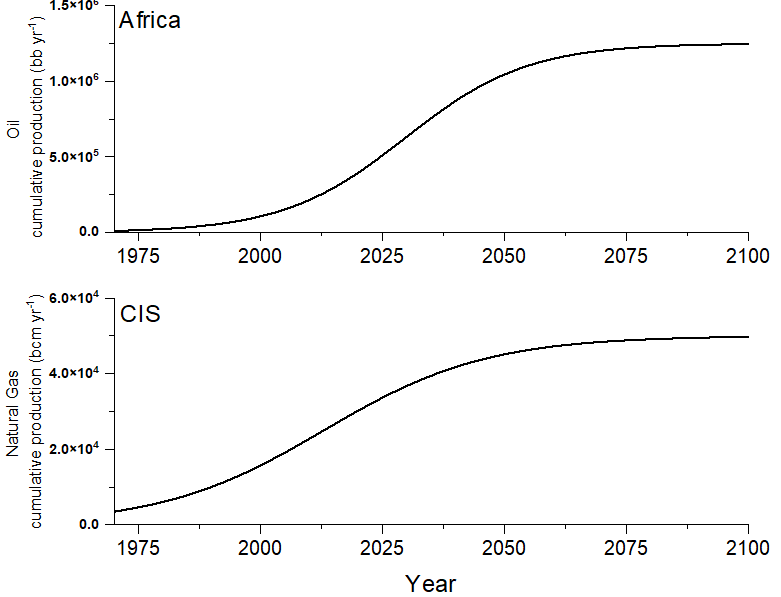
Figure 5 shows the cumulative production (N) from the base year by solving Eq. (1) and plotted, as examples, for oil production in Africa and natural gas in the CIS. Production N is a function of available reserves K and in the other cases we examine, masive reserves lead to a constant growth of production and therefore a plateu is not reached by 2100. Such curves enable us to quantify maximum production and specify it in time, so for example maximum oil production in Africa is 1.2x106 bb per year and is expected to be reached arround 2060.

4. Emissions

For the regions considered previously and for those which presented a good fit to a Hubbert curve, a study on projected production-based CO₂ emissions is conducted to give a first order estimation of the consumption of the available carbon budget under unconstrained extraction, as defined by the IPCC (Intergovernmental Panel on Climate Change) and shown in Table 4.

The regions studied cover 95% of worldwide fossil fuel emissions and are presented in Figure. 6. The results for future production calculated from Hubbert curves for each region and each fossil fuel were used in the estimation of emissions. The same projections were done considering the whole world using the available data [12]. In this way the major contributor regions in each fuel can be identified. In this study, each fossil fuel was considered separately in order to calculate its individual impact on the carbon budget.

For coal production, under unconstrained extraction, the Asia & Pacific region will contribute the greatest part of the coal-associated CO₂ emissions. Both China and Australia are among the countries with the greatest reserves in the world while bringing them to surface would lead to a substantial overshoot of the budget long before 2100. Luckily, actions to reduce coal consumption, principally from the closure of coal-fired power, are underway with Europe leading the adoption of mitigation strategies for 2050 [13].

Similar results are observed for oil-associated CO₂ emissions, this time with Middle East leading and being responsible for more than 50% of the associated production. Again, under unconstrained oil-production, the available carbon budget will be consumed by 2040 in the 2 ^oC scenario and by 2026 in the 1.5 ^oC scenario, and this takes no account of the contribution from coal.

In the case of natural gas, North America leads production and with it, associated CO₂ emissions. The available carbon budget, in the case of 2 ^oC scenario, will not be consumed by 2050 but there is barely any room left for other productive activities that produce CO₂ emissions, such as the oil and coal production analysed previously [14]. In contrast, in the case of 1.5 ^oC global warming scenario, there is an extensive overshoot. The above results indicate that, in order to stay below the suggested thresholds, coal production has to be eliminated well before 2050, oil production and therefore consumption has to be substantially decreased, while current natural gas production trends can be accepted for 2 ^oC scenario, but in the 1.5 ^oC, it too has to be decreased substantially. Such sharp reductions by 2050 are extremely difficult to achieve without extensive carbon capture and storage, so that for every mole of CO₂ emitted another one returns underground; this can provide us with much needed time for further mitigation actions.

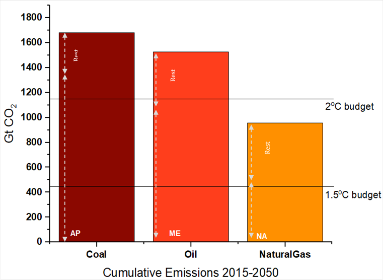
Table 4. Available carbon budget for the two global warming scenarios.

Scenario	Carbon Budget 2015-2100 (Gt CO2)	Reference
1.5 oC	420	[15]
2 oC	1170

5. Conclusions

The aim of this paper was the estimation of fossil fuel production from the main regions of the world, together with their associated carbon dioxide emissions. A first order determination of the carbon budget consumption was calculated for each fuel separately. Hubbert’s logistic function was matched to historical data to estimate future coal, oil and natural gas production. However, this model does not take into account future technological improvements and considers that nations exploit their full reserve potential with no artificial limitations to address, for instance, climate change concerns. For some regions, such as Europe, these assumptions are not correct and therefore Hubbert’s logistic function fails to fit the historical data.

These regions were excluded from the study. The CO₂ emissions for each fuel (coal, oil and natural gas) were estimated as if each fuel was used separately. In this way their individual effect on carbon budget can be determined. The results indicate that, for coal the available budget is exceeded well before 2050, with the major producer being the Asia & Pacific region. The same situation is observed for oil, in which unconstrained extraction results in a budget overshoot by 2040 in the 2oC scenario and 2026 in 1.5^oC scenario, even ignoring coal production. Natural gas extraction consumes 2/3 of the budget in the 2 ^oC scenario with North America being the main contributor. It is important to state that, if the production of fossil fuels continues as predicted, there is no available room for any productive activities that cause CO₂ emissions. To that extent, mitigation strategies such as carbon capture and storage, to further constrain production are essential.

Nomenclature

References

[1] IEA (2019), Natural Gas Information 2019, IEA, Paris. View Article
[2] IEA (2020), Global Energy Review 2020, IEA, Paris. View Article
[3] UNFCCC, 2015. Synthesis report on the aggregate effect of the intended nationally determined contributions. Available at: View Article
[4] Global Carbon Budget 2015, C. Le Quéré, R. Moriarty, R. M. Andrew, J. G. Canadell, S. Sitch, J. I. Korsbakken, P. Friedlingstein , et al. Earth Syst. Sci. Data, 7, 349–396, 2015 doi:10.5194/essd-7-349-2015. View Article
[5] IPCC Special Report on Renewable Energy Sources and Climate Change Mitigation, 2016. View Article
[6] K. Handayania , T. Filatova , Y. Krozera , P. Anugrah, Seeking for a climate change mitigation and adaptation nexus: Analysis of a long-term power system expansion. Applied Energy, Vol 262, 2020. View Article
[7] Hultman, N., Rebois, D., Scholten, M. & Ramig, C. The greenhouse impact of unconventional gas for electricity generation. Environ. Res. Lett. 6, 2011system expansion. Applied Energy, Vol 262, 2020. View Article
[8] K. Juhrich, CO2 Emission Factors for Fossil Fuels, Umwelt Bundesamt, 2016.
[9] BP Statistical Review of World Energy. Available at: View Article
[10] Sakiru Adebola Solarin, Luis A. Gil-Alana, Carmen Lafuente, An investigation of long-range reliance on shale oil and shale gas production in the U.S. market, Energy, Volume 195, 2020 oC. View Article
[11] European Union Energy roadmap 2050 available at: View Article
[12] Carbon dioxide (CO2) Emissions without Land Use, Land-Use Change and Forestry (LULUCF), in kilotonne CO2 equivalent, available at: View Article
[13] Dogan K., Hasan Ü. Y. Decarbonisation through coal phase-out in Germany and Europe — Impact on Emissions, electricity prices and power production, Energy Policy, 141, 2020. View Article
[14] Karvounis P., M. J. Blunt, A Hubbert Analysis on Natural Gas Production of the Top Producers. How the Carbon Budget Is Affected Under Unconstrained Extraction, 5th World Congress on Civil, Structural, and Environmental Engineering (CSEE'20).
[15] Masson-Delmotte, V., P. Zhai, H.-O. Pörtner, D. Roberts, J. Skea, P.R. Shukla, A. Pirani, W. Moufouma-Okia, C. Péan, R. Pidcock, S. Connors, J.B.R. Matthews, Y. Chen, X. Zhou, M.I. Gomis, E. Lonnoy, T. Maycock, M. Tignor, and T. Waterfield, IPCC, 2018: Summary for Policymakers. In: Global Warming of 1.5°C. An IPCC Special Report on the impacts of global warming of 1.5°C above pre-industrial levels and related global greenhouse gas emission pathways, in the context of strengthening the global response to the threat of climate change, sustainable development, and efforts to eradicate poverty, World Meteorological Organization, Geneva, Switzerland, 32 pp.