Journal of Fluid Flow, Heat and Mass Transfer (JFFHMT)

ISSN: 2368-6111

Nomenclature

1. Introduction

Condensation is the change of the physical state of matter from the gas phase into the liquid phase due to the removal of heat. It is an important process in many industrial applications including, nuclear reactors, electric cooling, metallurgical processes, biochemical processes, etc. The steam bubble condensation process is critical in nuclear reactors as it controls the reactivity and thus influences the safety of the reactor [1]. Regardless of its application in various industries, the condensation phenomenon is slightly complicated as it undergoes both heat and mass transfer processes. Further, the interface between vapor and liquid regions changes irregularly, and that increases the difficulty in interpreting the mass transfer.

In the year 1987, Kamei and Masaru had conducted experiments to understand the condensation of a saturated vapor bubble placed in sub-cooled liquid [2]. Their results explained the various shape changes observed during condensation at different sub-cooling temperature and operating pressure. Bubble behaviour in subcooled flow boiling of water at low pressures and low flow rates were studied by Prodanovic et al at 2002 [3]. In 2011, Kim and Park consolidated the interfacial heat transfer of condensing bubble in subcooled boiling flow at low pressure [4]. Evaporation condensation-induced bubble motion were studied by Nikolayev et al at 2017 [5]. All the works conclude that the difference in the local temperature gradient near the interface could be one of the prime reasons for the change in the bubble shape during condensation process.

Though the results obtained by the experimental approach were reliable, it involves a huge effort for the experimental setup. The accurate prediction of mass transfer at the interface is also not easily possible by experiments, whereas a numerical approach can allow these details to derive with relative ease. Many researchers had worked on numerical approach to solve condensation problem. In 2014, Sun et al modelled the mass transfer using phase change equations through UDF and explained the change in bubble lifetime with respect to initial bubble diameter [6]. The bubble lifetime is considered the time it takes for the bubble to condense completely. The researchers like Zeng et al and Samkhaniani et al tried to capture interface by calculating the gradient of volume fraction and smoothed the curvature to control the spurious currents [7, 8]. Another prominent reference in this area is the work done by Tian et al, who solved the steam bubble condensation problem using a moving particle semi-implicit (MPS) method [9]. The work explained the influence of gravity and bubble shape changes due to system pressure.

In the case of condensation, the interface capturing is very crucial to obtain a proper shape of the bubble. The VOF and multi-fluid VOF models are generally used when the shape of the interface is of interest, and the interfacial length scale is larger than the computational grid. In the standard VOF method, the momentum and temperature equations are shared between the phases. Whereas the multi-fluid VOF comes under the Eulerian models in which separate equations are solved for each phase, and this permits a sharp interface modelling. The multi-fluid VOF model is adopted in the present study as it is a better choice for bubble flows. In Ansys-Fluent, one of the methods to solve the condensation phenomenon is by using the Thermal Phase Change (TPC) model. The TPC model is a volumetric phase change model in which mass transfer coefficients are governed by the chosen heat transfer mechanism.

2. Overview of Numerical Methods

2.1 Governing Equations for Multifluid VOF Model

The multi-fluid VOF model provides a framework to couple the VOF and Eulerian multiphase models and allows the use of discretization schemes to solve sharp interfaces. The model is further equipped to overcome some limitations of the VOF model that arise due to the shared temperature and velocity formulation.

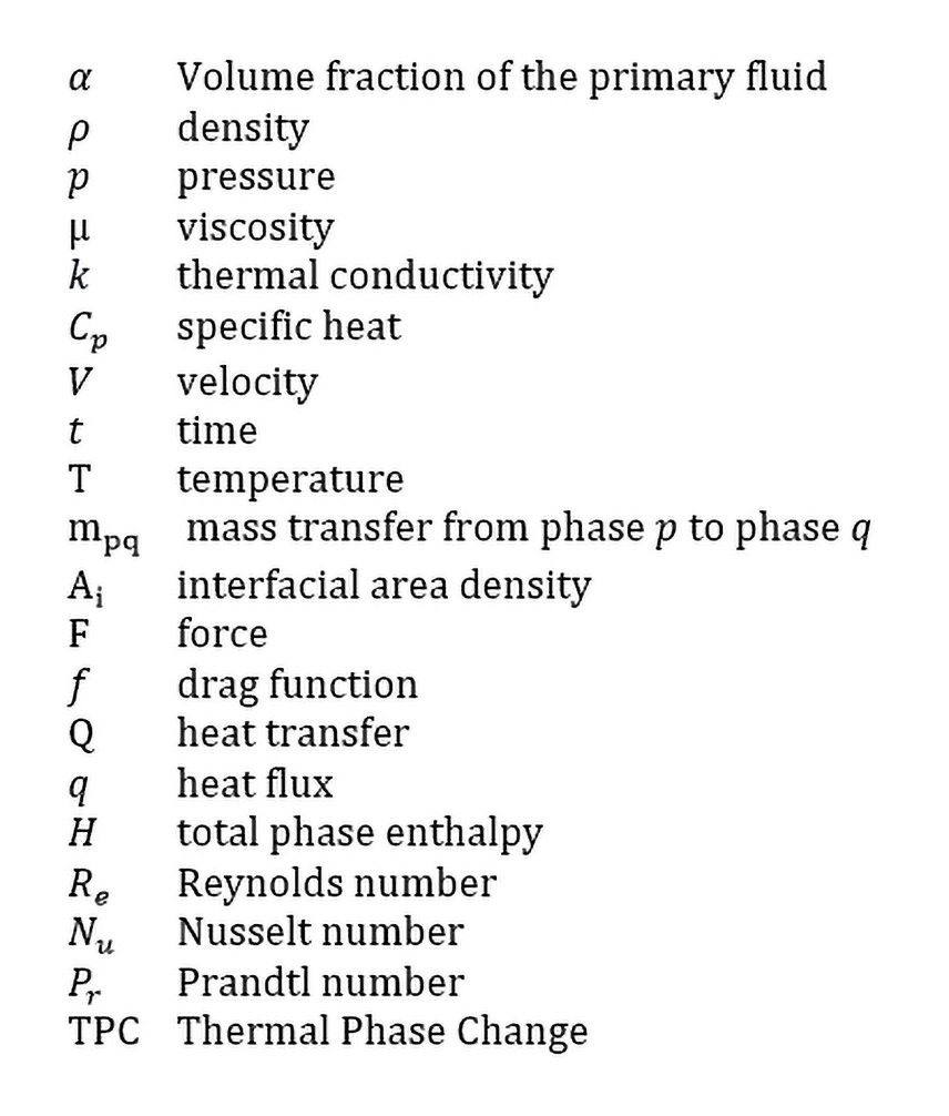
The governing continuity equation is defined as follows:

ρ_rq is the phase reference density used in the discretization of continuity and VOF equations. V_q is the velocity of phase q and m_pq is the mass transfer from phase p to phase q.

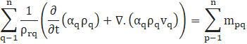
The interface is modelled via volume fraction. The volume of a phase is defined as:

Where,

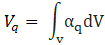
The VOF equation of phase q is defined as:

The momentum equation is defined as:

is the q^th phase shear-strain tensor. F_lift,q is the lift force and F_vm,q is the virtual mass force of the q^th phase. p is the pressure shared by all phases and R_pq is the interaction force between phases.

The interaction between the phases is modelled via drag. In this case, the symmetric drag law is applied between the immiscible fluids. The symmetric drag law coefficient can be represented as follows:

If,  

R_e is the Reynolds number. f is the drag function. μ is averaged viscosity.

Finally, the energy equation is defined as follows:

h_q is the specific enthalpy of q^th phase, q_q is the heat flux, Q_pq is the intensity of heat transfer between the phases, h_qp is the interface enthalpy and j_jq is the diffusive flux of the phase q.

2. 2. Evaporation and Condensation Modelling

In the evaporation or condensation process, the mass transfer occurs between liquid and gas phases at the interface. The TPC model is one of the models available in ANSYS Fluent solver to account for the mass transfer.

The TPC model works in the Eulerian multiphase framework. It applies the two-resistance approach where a separate heat transfer process is considered for either side of the phase-interface with different heat transfer coefficients.

The heat transfer from the interface to the liquid phase is given by:

The heat transfer from the interface to the vapor phase is given by:

Where h_l and h_v are the heat transfer coefficients of liquid and vapor, respectively. H_ls and H_vs are the enthalpies of liquid and vapor phases. C_l and C_v are the scaling factors. T_s is the saturation temperature. A_i is the interfacial area density for the phase i.

Heat or mass cannot be stored on the phase interface; hence heat balance must need to be satisfied.

From the above heat transfer equations, the overall mass transfer for condensation can be expressed as follows:

In condensation,    , therefore:

In the presence of mass transfer, H_l and H_vare total phase enthalpies and can be expressed as:

T_ref is the reference temperature and H (T_ref) is the standard state enthalpy at T_ref.

In the TPC model, the mass transfer process is completely governed by the interphase heat transfer process and no further calibration is required, therefore, this model is generally recommended for the condensation problems.

2.3. Modelling of Heat Transfer Coefficient

In some cases, the interface heat transfer coefficient (h_l and h_v in Eq. 8 and Eq. 9) cannot be solved accurately with the overall heat transfer coefficient. The two-resistance model is applied to separate the heat transfer processes having two different heat transfer coefficients on the either side of the phase interface. The heat transfer coefficient is calculated from the Nusselt number (Nu) using the following equation.

Where h_lv is the heat transfer coefficient, k_l is the thermal conductivity of the liquid, N_u is the Nusselt number, and d is the diameter of the bubble.

Further, the Nusselt number is calculated from the relation of Reynolds number and Prandtl number using the following formulations:

The Ranz-Marshall model is widely used to calculate N_u especially when the flow is laminar.

2.4. Interfacial Area Density Modelling (A_i)

The interfacial area density (A_i) in the Eq. 8 and Eq. 9 is calculated by taking the magnitude of the gradient of volume fraction α.

The volume integral of the area density must be equal to the real surface area of the interface. The accurate calculation of interfacial area density plays a significant role to calculate heat and mass transfer in the TPC model. The interfacial region between liquid and vapor changes very irregularly, therefore, it is crucial to maintain a smooth distribution. In the present work, two different smoothing methods for area density calculation are studied in detail.

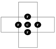
2.4.1 Cell-based smoothing

In this method, the interfacial area density is calculated by considering the face-connected neighbours of the active cell, as shown in Figure 1. Here, the volume fraction used to obtain the interfacial area is the area-weighted average of the volume fraction at the surrounding faces.

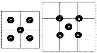
2.4.2 Node-based smoothing

This method possesses a larger stencil compared to the cell-based smoothing. The interfacial area density is calculated by considering the cells connected neighbours of each node of the active cell, as shown in Figure 2. First, the nodal values of volume fraction are constructed from the volume-weighted average of the cell values surrounding the nodes. Then these node values are arithmetically averaged (based on the number of total nodes of the cell) to provide a smoothed volume fraction field for each cell.

The above two methods are compared for a circular (2D) and spherical (3D) shapes and predicted areas are verified with the analytical value.

Figure 3 shows, the node-based smoothing method provides a smoother area density. Table 1 shows a comparison of predicted area with the analytical area for both the methods. It can be observed that the node-based smoothing method provides less error compared to the cell-based smoothing method. It is also important to have a smoothed interface as it controls the abrupt change of volume fraction, otherwise it might arise errors in calculating normal vectors and curvature of the interfacial forces.

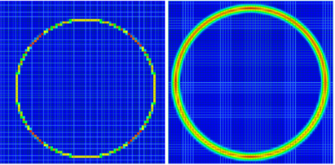
Table 1. Interfacial area comparison with analytical data.

Bubble shape details	Analytical area [m²]	Cell based method error %	Node based method error %
Circle (r = 7.5 [mm], 2D planar)	0.0471	0.23	0
Circle (r = 7.5 [mm], 2D axisymmetric)	0.0007065	2.19	0.1
Sphere (r =7.5 [mm], 3D)	0.0007065	2.3	0.18

3. Validation of Vapor Bubble Condensation

3.1. Problem Description

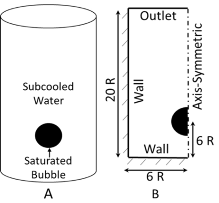
The objective of this study is to simulate the condensation phenomenon of a single water vapor bubble placed in sub-cooled liquid water by using the Thermal Phase Change model and multi-fluid VOF method implemented in ANSYS Fluent solver. A spherical shaped water vapor bubble is patched in a cylindrical pool filled with sub-cooled water, as shown in Figure 4 (A). Exploiting the axisymmetric nature of the domain, only a 2D rectangular section with axis symmetry is used for this simulation. The domain extent is dependent on the initial radius of the bubble (20R ×6R) as shown in Figure 4 (B). The various initial sizes of the bubble with a diameter (2R) of 1 mm, 3 mm, 5 mm, 10 mm, 13.5 mm, 14 mm, and 15 mm are patched in the rectangular domain with a distance of 6R from the bottom wall. The top boundary is a pressure outlet with ambient pressure. Axisymmetric is the axis and the rest of the boundaries are considered as the adiabatic walls.

The properties of water and water-vapor, especially density (ρ), specific heat (C_p), thermal conductivity (k), and viscosity (µ) change with temperature (T) and system pressure (P) are shown in Table 2 and Table 3, respectively.

Table 2. Properties of water liquid at different pressure and temperature.

P [MPa]	T [K]	ρ [kg/m3]	Cp [J/kgK]	k [W/mK]	µ [Kg/ms]
0.1	350	973.73	4194.5	0.668	3.5e-4
	353	971.88	4196.6	0.669	3.53e-4
	360	967.40	4202.3	0.673	3.26e-4
0.2	373	958.50	4215.3	0.679	2.82e-4
	375	957.06	4217.6	0.679	2.76e-4
0.4	395	941.70	4246.1	0.683	2.28e-4

Table 3. Properties of water vapor at different pressure and temperature.

P [MPa]	T [K]	ρ [kg/m3]	Cp [J/kgK]	k [W/mK]	µ [Kg/ms]
0.1	400	0.554	2009.3	0.027	1.32e-5
	373	0.597	2079.9	0.025	1.2e-5
	390	0.569	2027.1	0.026	1.29e-5
0.2	393	1.129	2178.2	0.027	1.29e-5
	405	1.093	2116.9	0.0282	1.34e-5
0.4	425	2.112	2260.5	0.031	1.41e-5

3.2. Case Setup

A computational grid is created with uniform structured quadrilateral elements. A grid independence study is carried out for the case with 5 mm initial bubble diameter, on four different grids with the element size of 0.1mm x 0.1 mm, 0.07 mm x 0.07 mm, 0.05 mm x 0.05 mm and 0.03 mm x 0.03 mm. The bubble lifetime is compared with the Kamei experimental results. The case with the element size of 0.05 mm x 0.05 mm produced grid independent results thus, it is considered for the further studies. The orthogonal quality of the mesh is close to 1.

The other conditions in the present work are kept consistent with the study done by Sun et al [6]. The flow is considered as laminar. Gravity is switched on to consider buoyancy effect. Surface tension is modelled to achieve the proper shape of the bubble during condensation. Water is considered as the primary liquid phase and water-vapor as the secondary gas phase. The properties of liquid water change with temperature, a piecewise linear function is used to accommodate that change. The transient simulations are carried out using a pressure-based solver with a time step size of 10e-06 s. The phase coupled SIMPLE solver is used as it is best suited for the Eulerian models. The PRESTO! (PREssure STaggering Option) scheme is used for pressure discretization. The momentum and energy are discretized using first order upwind schemes to achieve better convergence. The volume fraction cut off is taken as 10e-06.

3.3. Results and Discussion

The impact of scaling factors in the TPC model is studied and presented. The influence of area density calculation is analysed further. The bubble shape change during the condensation process is studied in detail. The bubble lifetime variations due to initial bubble diameter, system pressure and subcooling temperature are validated against experimental and previously published data.

3.3.1. Influence of Scaling Factors in TPC model

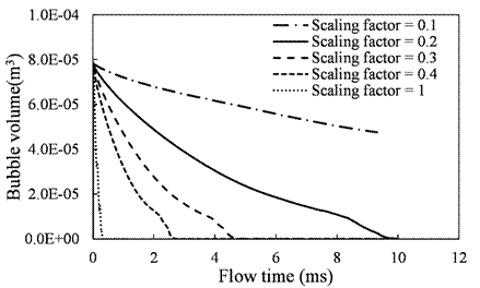
The thermal phase change model uses scaling factors (C_l and C_v) to calculate the heat transfer from the interface to the liquid phase or gas phase as shown in Eq.8 and Eq.9. The default value of these scaling factor is 1. To understand the influence of scaling factors on the mass flow, a case study is conducted on a bubble with 5 mm of initial diameter. The bubble lifetime is compared for different scaling factors as shown in the Figure 5. The experimental value for the lifetime of 5 mm initial diameter bubble is 9.5 ms [2]. It is observed that the bubble lifetime is over predicted for scaling factors of 1, 0.4 and 0.3; whereas it is under predicted for the scaling factor of 0.1. The prediction of bubble lifetime is close compared to experimental when scaling factor of 0.2 is used. Therefore, the scaling factor of 0.2 is fixed for all other cases and the idea is to achieve results close to experimental by using the same scaling factor irrespective of the change in initial bubble diameters, different operating pressures, and temperatures.

3.3.2. Influence of Interfacial Area Calculation Method on Bubble Life

A case study is done to check the influence of interfacial area calculation methods. The analysis is conducted on the bubbles with initial diameter of 13.5 mm and 14 mm, at atmospheric pressure and subcooling temperature of 20 K. The results obtained from simulation are compared to the Kamei’s experimental results [2]. It is observed that the node-based smoothing method shows 0.8% of error compared to 2.9% using the cell-based smoothing method for the bubble with initial diameter of 13.5 mm. The error percentage for the bubble with initial diameter of 14 mm is 2.9% for the node-based smoothing method and 7 % for the cell-based smoothing method, respectively. Therefore, the node-based smoothing method is used for the further case studies.

3.3.3. Bubble Shape Change during the Condensation Process

During the condensation process, the bubble shape is controlled by the drag force, buoyancy, surface tension, and the inertial force induced by the liquid on the bubble. To understand the bubble shape change during condensation, a case study is carried out on the bubbles having an initial diameter of 5 mm, 10 mm, 15 mm, and 18 mm. The analysis is conducted at the atmospheric pressure and subcooling temperature of 20 K. Figure 6 shows the bubble shape history at every 2 milliseconds for the bubble of 18 mm initial diameter. The bubble shape contours obtained from the numerical solution are validated against the images of Kamei’s experiment [2] and published data by Tian et al with the MPS method [9]. The bubble shapes at the intermittent time shows a good match with the experiment.

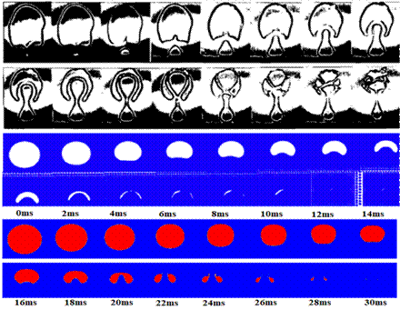
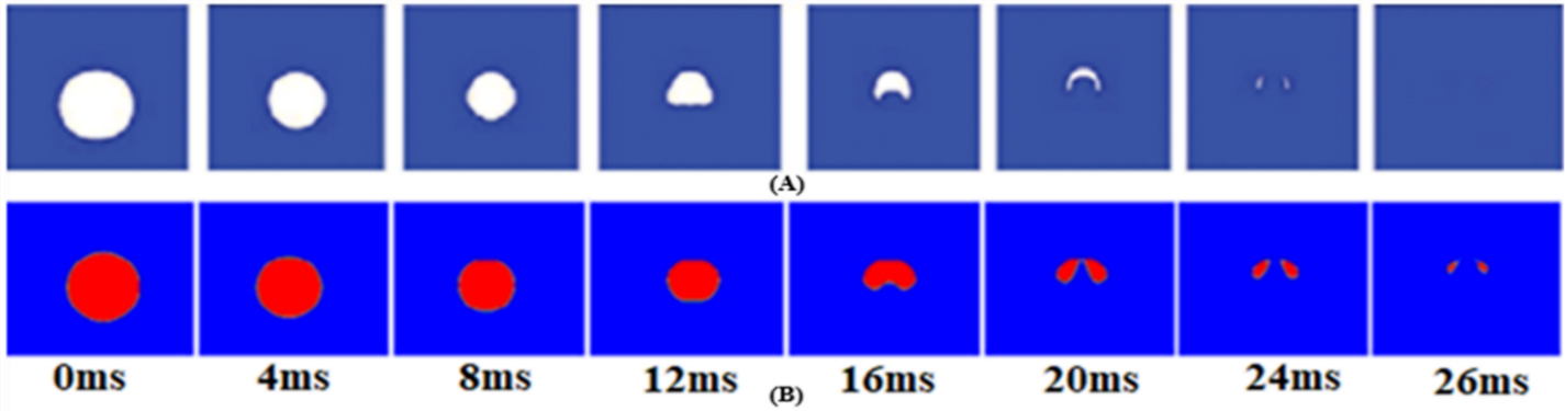
Figure 7 shows the bubble shape history at every 4 milliseconds for the bubble of 15 mm initial diameter and the results are compared with Sun et al results [6]. In both cases, the bubble shape remained circular during the initial stage of condensation. After a certain time, the bubbles get expanded forming into a disk shape and broke into two smaller bubbles before they completely condensed. The analysis is further extended to the bubbles with initial diameter of 5 mm and 10 mm, maintaining the ∆T as 20 K and the system pressure as 1 atm. It is found that the bubble shape changes are very similar to the 18 mm initial diameter bubble.

3.3.4. Bubble Lifetime Vs Initial Bubble Diameter

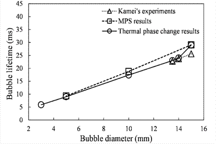
The bubble lifetime is considered as the total time taken for the vapor bubble to disappear completely due to condensation. A case study is conducted to understand the impact of the initial bubble diameter on the bubble lifetime. The analysis is carried on the bubbles with initial diameters of 3 mm, 5 mm, 10 mm, 13.5 mm, 14 mm, and 15 mm. The system pressure and temperature ∆T are considered as 1 atm and 20 K, respectively. The results obtained from the current simulation are validated against the experiment [2] and compared with the data published by Tian et al solved with MPS method [9]. The results are shown in Figure 8 and it could be observed that the variation of bubble lifetime with respect to initial bubble diameter is almost linear. The lifetime obtained from TPS method matches very well with the experiment (error around 1%) for the bubbles with an initial diameter of 13.5 mm and 14 mm. The lifetime of bubble is overpredicted (error around 13%) for the initial diameter of 15 mm compared to experimental, but the same trend is observed with the numerical results obtained from MPS method as well, which needs a further investigation.

3.3.5. Bubble Lifetime Vs System Pressure

A case is validated to understand the influence of the system pressures on the bubble lifetime. The analysis is done on a bubble with an initial diameter of 1 mm and temperature ∆T of 30 K. The system pressure is varied to 0.1 MPa, 0.2 MPa, and 0.4 MPa. Material properties have been changed according to the pressure variation. Figure 9 shows the variation of bubble lifetime to system pressure, the results are validated with the data published by Pan et al [10].

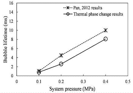
The higher system pressure results in higher vapor density and volumetric latent heat, thus the bubble lifetime increase with the increase in system pressure. The bubble lifetime obtained from the TPC method is very close to the results published by Pan et al when system pressure is 0.1 MPa. When system pressure is increased to 0.2 MPa and 0.4 MPa, the bubble lifetime obtained from TPC method is underpredicted by 19% which again needs more investigation.

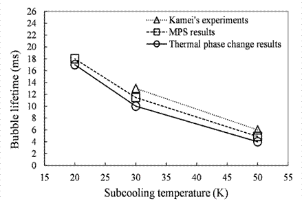
3.3.6. Bubble lifetime Vs Subcooling temperature

In this case study, the effect of subcooling temperature is evaluated and results are validated against the experiment [2]. The results are also compared with the data published by Tian et al solved with MPS method [9] and with the data published by Pan et al [10]. The first case is carried out on the bubble with initial diameter of 10 mm and at 1 atmospheric pressure. The temperature ∆T is varied to 20 K, 30 K and 50 K. The bubble lifetime decreases with the increase in subcooling temperature due to the enhancement of mass and energy transfer between both the phases. The results obtained from the TPC model depicts a reasonable match with the experiment and results obtained from the MPS method as shown in Figure 10.

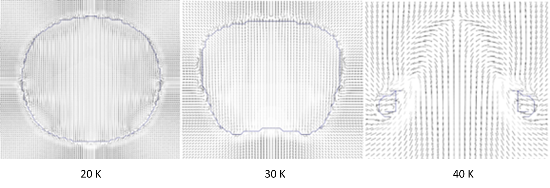
Another case is solved with an initial diameter of bubble as 1 mm and temperature ∆T as 40 K. The results are compared with the data published by Pan et al [10] which shows a very good match with an error of less than 5%. The case is extended for the temperature ∆T as 20 K, 30 K. The velocity vectors around the bubble at 0.2 millisecond are shown in Figure 11, this clearly depicts the effect of temperature on bubble shape and flow field around it.

4. Conclusion

In the present study, the condensation phenomenon of a single vapor bubble in the sub-cooled water medium is numerically simulated in ANSYS Fluent CFD solver using the Multi-fluid VOF and the Thermal phase change model. Further the different approaches to calculate the interfacial area density are evaluated which play a significant role in the accurate prediction of mass transfer during the condensation process. It is concluded that the node-based smoothing method for interface modelling provides a larger stencil compared to the cell-based smoothing method and provides more accurate prediction of the area.

A validation study is carried out with multiple initial bubble diameters and the change in shape for the bubble during the condensation process is compared with experimental images. The images obtained from numerical solution show a reasonable match with experimental. It is observed that the bubble with larger initial diameter tends to maintain a circular shape for a longer period before it converts into a mushroom like structure and break down into two smaller bubbles. The bubble with smaller initial diameter tends to change the shape quickly and break down into two smaller bubbles before getting condensed entirely. The lifetime of the bubble is also obtained for different initial diameters and validated against experimental and previously published data with a close match. The validation is further extended for different system pressures and sub-cooling temperatures. The lifetime of the bubble with an initial diameter of 1 mm and temperature difference ∆T of 30K is compared with the previously published paper for different system pressures. It is observed that the bubble lifetime increases with the increase in system pressure. The results show a similar trend but the TPC results are under predicting the bubble lifetime compared to the reference results published by Pan et al [10] which provides a scope for further investigation. Two cases are considered to show the effect of subcooling temperature, the first case is simulated with the initial diameter of 10 mm and initial pressure if 1 atm for different temperature differences and the results are validated against experimental. The second case is solved for a bubble with an initial diameter of 1 mm, temperature ∆T as 40 K and results are compared with the data published Pan et al [10]. In both cases, the bubble lifetime decreases with an increase in subcooling temperature and the results are close to experimental or reference data. Thus, it can be concluded that the steam bubble condensation phenomenon could be numerically simulated with close accuracy using the TPC method implemented in ANSYS Fluent along with the node-based smoothing method for interfacial area calculation. The node-based smoothed interfacial area is superior to the default interfacial area and will be accounted for in the future development cycle of Ansys Fluent.

References

[1] Yadigaroglu, G. (2005). Computational fluid dynamics for nuclear applications: from CFD to multi-scale CMFD. Nuclear Engineering and Design, vol. 235, no. 2-4, pp. 153–164. View Article
[2] Kamei, S., and Hirata, M. (1987). Condensing phenomena of single vapor bubble into subcooled water, 1. Nippon Kikai Gakkai Ronbunshu, B Hen, vol. 53, no. 486, pp. 464–469. View Article
[3] Prodanovic, V., Fraser, D., and Salcudean, M. (2002). Bubble behavior in subcooled flow boiling of water at low pressures and low flow rates. International Journal of Multiphase Flow, vol. 28, no. 1, pp. 1–19. View Article
[4] Kim, S.-J., and Park, G.-C. (2011). Interfacial heat transfer of condensing bubble in subcooled boiling flow at low pressure. International Journal of Heat and Mass Transfer, vol. 54, no. 13-14, pp. 2962–2974. View Article
[5] Nikolayev, V. S., Garrabos, Y., Lecoutre, C., Pichavant, G., Chatain, D., and Beysens, D. (2017). Evaporation condensation-induced bubble motion after temperature gradient set-up. Comptes Rendus Mécanique, vol. 345, no. 1, pp. 35–46. View Article
[6] Sun, D., Xu, J., and Chen, Q. (2014). Modeling of the evaporation and condensation phase-change problems with fluent. Numerical Heat Transfer, Part B: Fundamentals, vol. 66, no. 4, pp. 326–342. View Article
[7] Zeng, Q., Cai, J., Yin, H., Yang, X., and Watanabe, T. (2015). Numerical simulation of single bubble condensation in subcooled flow using OpenFOAM. Progress in Nuclear Energy, vol. 83, pp. 336–346. View Article
[8] Samkhaniani, N., and Ansari, M. (2016). Numerical simulation of bubble condensation using CF-VOF. Progress in Nuclear Energy, vol. 89, pp. 120–131 View Article
[9] Tian. W. X, Ishiwatari. Y., Ikejiri, S., Yamakawa, M., and Oka, Y. (2010). Numerical computation of thermally controlled steam bubble condensation using moving particle semi-implicit (MPS) method. Annals of Nuclear Energy, vol. 37, no. 1, pp. 5–15. View Article
[10] Pan, L.-m., Tan, Z.-w., Chen, D.-q., and Xue, L.-c. (2012). Numerical investigation of vapor bubble condensation characteristics of subcooled flow boiling in vertical rectangular channel. Nuclear Engineering and Design, vol. 248, pp. 126–136. View Article