Journal of Fluid Flow, Heat and Mass Transfer (JFFHMT)

ISSN: 2368-6111

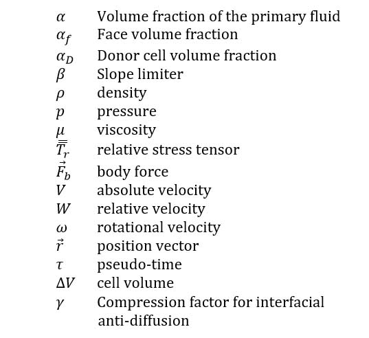
Nomenclature

1. Introduction

Fiberglass is extensively used as a filtration and an insulation material in construction, manufacturing, automotive, and aerospace industries due to properties such as high thermal and noise insulation, low weight, and low installation cost [1]. The fiberglass manufacturing process comprises of fiber extrusion and fiber attenuation: shear elongation, thinning, and solidification using a rotary spinner. In this process, highly viscous molten glass is made to spin at a very high speed. Due to high centrifugal forces, molten glass is extruded out of the spinner orifices and it is then attenuated by high-speed air to manufacture fiberglass. Visually, this process is very similar to the process used to manufacture cotton candy.

Several authors have studied the fiberization process of molten materials. Bizjan et al investigated the molten fructose sugar fiberization process and developed a 0D modelling approach and validated it experimentally [2]. Kraševec et al. carried out experiments on the glass wool fiberization process and developed regression models for fiber properties based on the operating parameters [3]. John J. McKetta Jr analysed the key process parameters that affect the glass film thickness on the spinner wall [4]. W. Arne et al. developed a combination of various 1D-2D modelling techniques for single fiber formation and fiber-fiber interactions [5,6]. Bizjan et al applied the Volume-of-Fluid (VOF) method for numerical modelling of ligament growth on a spinning wheel for mineral wool cascade fiberization process [7].

The previous studies are mostly based on experimental methods or reduced order modelling. There is a limited work available on the detailed numerical modelling of the complete rotary fiberization process. An accurate understanding of the spinning process is the starting point towards improving fiber quality and size distribution. This work focuses on the analytical and numerical aspects of fiberization process which includes filling, spinning, film formation, and extrusion through spinner orifices. A steady-state CFD solution methodology is developed for efficiently simulating this process using the VOF method. The pseudo-transient method is used to enhance the numerical robustness of the steady-state solver by improving the diagonal dominance. The coupled solution of the continuity and momentum equations, along with stabilization methods help to increase the solution stability with an aggressive pseudo-time step size. The interfacial anti-diffusion is used to achieve a crisp interface by reducing the numerical diffusion which arises from the volume fraction discretization schemes [8]. All the CFD validation case studies presented in this work are performed using the Ansys Fluent software.

2. Overview of Numerical Methods

2.1 Governing Equations for VOF Modelling in the Relative Frame of Reference

The governing equations for CFD are based on the conservation of mass, momentum, and energy which are solved using the Finite Volume Method (FVM). The equations are formulated in the relative frame as it offers faster convergence and reduces the round-off errors for the rotating flow problems considered in this work as compared to the absolute velocity formulation. The volume fraction equation is solved to identify the interfaces between immiscible fluids. The summation of the volume fraction for all the fluids should be equal to one. The volume fraction equation in the absence of mass sources is given as:

The continuity equations for a steady state flow can be formulated as:

For VOF model, a single momentum equation is solved throughout the domain and the resulting velocity field is shared among the phases. The momentum equation for a steady state flow in the relative formulation is given as:

Relative velocity , for pure rotating flow with constant rotational velocity is defined as:

Where, are represented as, fluid volume fraction, density, pressure, absolute velocity, rotational velocity, position vector in rotating frame, relative stress tensor, body force and pseudo-time respectively. The properties used in the momentum equation are volume-weighted averaged properties.

2. 2. Pseudo Transient Method

The pseudo-transient method is a time marching technique to achieve a steady state solution in a robust manner using the pseudo time step size. Robustness of the steady-state calculations is improved due to the added diagonal dominance from pseudo-transient terms. It also serves the purpose of providing a local implicit under-relaxation as shown below in a generalized, governing equation.

Where, ρ is the density, ΔV is the cell volume, ϕ_p and ϕ_nb are the solution variables at the cell center and neighboring cells, a_p and a_nb are coefficients of central and neighbouring cells, ∆τ is the pseudo time step size and b is the source term.

This method can be assisted with stabilization techniques such as dual pseudo-time stepping, and smoothing methods to improve the solution stability with aggressive pseudo-time step size.

2. 3. Pressure Velocity Coupling

The pressure based coupled approach solves the momentum and continuity equations together and hence it provides a robust and superior performance as compared to the segregated solution approach. A full implicit coupling is achieved through an implicit discretization of the pressure gradient terms in the momentum equations, and an implicit discretization of the face mass flux, including the Rhie-Chow pressure dissipation terms [8].

2.4. Compressive Scheme for volume fraction discretization

The compressive scheme is a second order scheme based on the slope limiters [8].

Where,  is face volume fraction,  is donor cell volume fraction, is the slope limiter with the maximum value of 2,   is interface normal for donor cell and  is the position vector between donor cell centroid and face centroid [8].

2.5. Interfacial Anti-Diffusion

The interfacial anti-diffusion treatment attempts to suppress the numerical diffusion that can arise from the volume fraction advection schemes, especially for the mesh with coarse cells, high aspect ratio or with a large cell volume jump in the vicinity of a fluid-fluid interface.

A diffusion source term with a negative diffusion coefficient is added in the volume fraction equation for the numerical sharpening of the interface [8].

Where,

   is the compression velocity in the direction normal to the interface, and and γ is the compression factor varying between 0 and 1, where, γ =0 means no compression and γ =1 means maximum compression.

3. Validation Studies

The complex physics of molten glass flow in a rotating spinner is resolved using several fundamental case studies, following a step by step approach. Firstly, validations are done against the analytical solution for 2-phase viscous Poiseuille flow and rotating viscous flow in a closed domain. Thereafter, modelling and validation of the full fiberization spinner is carried out. Simplification is done by using a 2D axisymmetric swirl representation of the actual fiberization spinner geometry as it can capture the full physics with a reduced computational effort.

The pressure based coupled solver is used along with the pseudo-transient method with an automatic pseudo-time step size. The Compressive scheme is used for the volume fraction discretization along with interfacial anti-diffusion. PRESTO! (PREssure STaggering Option) is used for the face pressure interpolation whereas, 2nd order upwind discretization schemes are used for the momentum and swirl equations [8]. The laminar viscous model is applied as the molten glass has a creeping flow regime due to very high viscosity.

3.1. Case Study 1: Two-Phase Poiseuille Flow

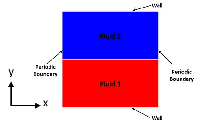
The objective of this case study is to validate the two-phase Poiseuille flow for highly viscous fluids which is one of the key physics in the glass fiberization process. Two layers of different fluids are subjected to the same pressure gradient in the horizontal direction as shown in the Figure 1. The flow domain and boundary conditions are shown in Figure 2. The analytical velocity profiles are derived in different fluids after satisfying the boundary conditions at the wall and interface. This case study is a good demonstration of how well the shear stress is resolved at the interface for highly viscous fluids using the VOF method.

The final velocities of fluid 1 and fluid 2 are given as,

Where,

Where, μ₁ and μ₂ are viscosities of fluid 1 and fluid 2, p is the pressure,  is the pressure gradient in the x direction.

In this case study, a 2D square domain of 0.02 [m] x 0.02 [m] is half-filled with fluid 1 as shown in Figure 2. The computational grid comprises for 25.6K quad-structured mesh elements. The top and bottom boundaries are walls and side boundaries are streamwise periodic with a pressure gradient of 10.62 [Pa/m]. The velocity profiles are independent of density; therefore, it is taken as 10 [kg/m^3] for both the fluids. In the first case, μ₁ and μ₂ are considered as 5e-4 [kg/m-s] and 1.85e-5 [kg/m-s] respectively to get a viscosity ratio of 27 whereas in the second case, μ₁ and μ₂ are considered as 1e5 [kg/m-s] and 1e-3 [kg/m-s] to achieve a viscosity ratio of 1e8.

The velocity profiles are validated against the analytical solution for low and high viscosity ratio cases as shown in the Figure 3 and Figure 4, respectively. It demonstrates that the current modelling methodology can resolve the interfacial shear stresses and obtain the velocity profiles accurately for fluids with high viscosity ratio.

3.2. Case Study 2: Highly Viscous, Two-Phase Flow in a Closed Rotating Tank

The objective of this case study is to validate the CFD predicted free surface shape and pressure distribution against the analytical solution for a highly rotating and highly viscous two-phase flow in a closed domain.

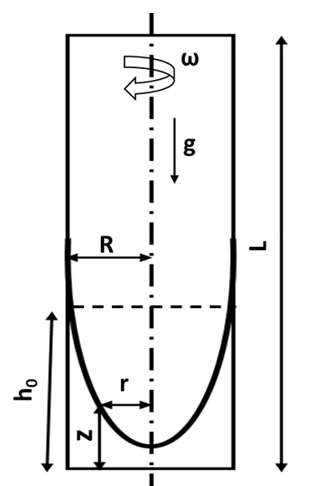
A rotating cylindrical tank is partially filled with the molten glass as shown in the Figure 5. All the walls of the tank are assumed to be adiabatic. The cylinder is made to spin about its vertical axis. At the final steady-state, the liquid will move as a rigid body forming a distinct free surface profile.

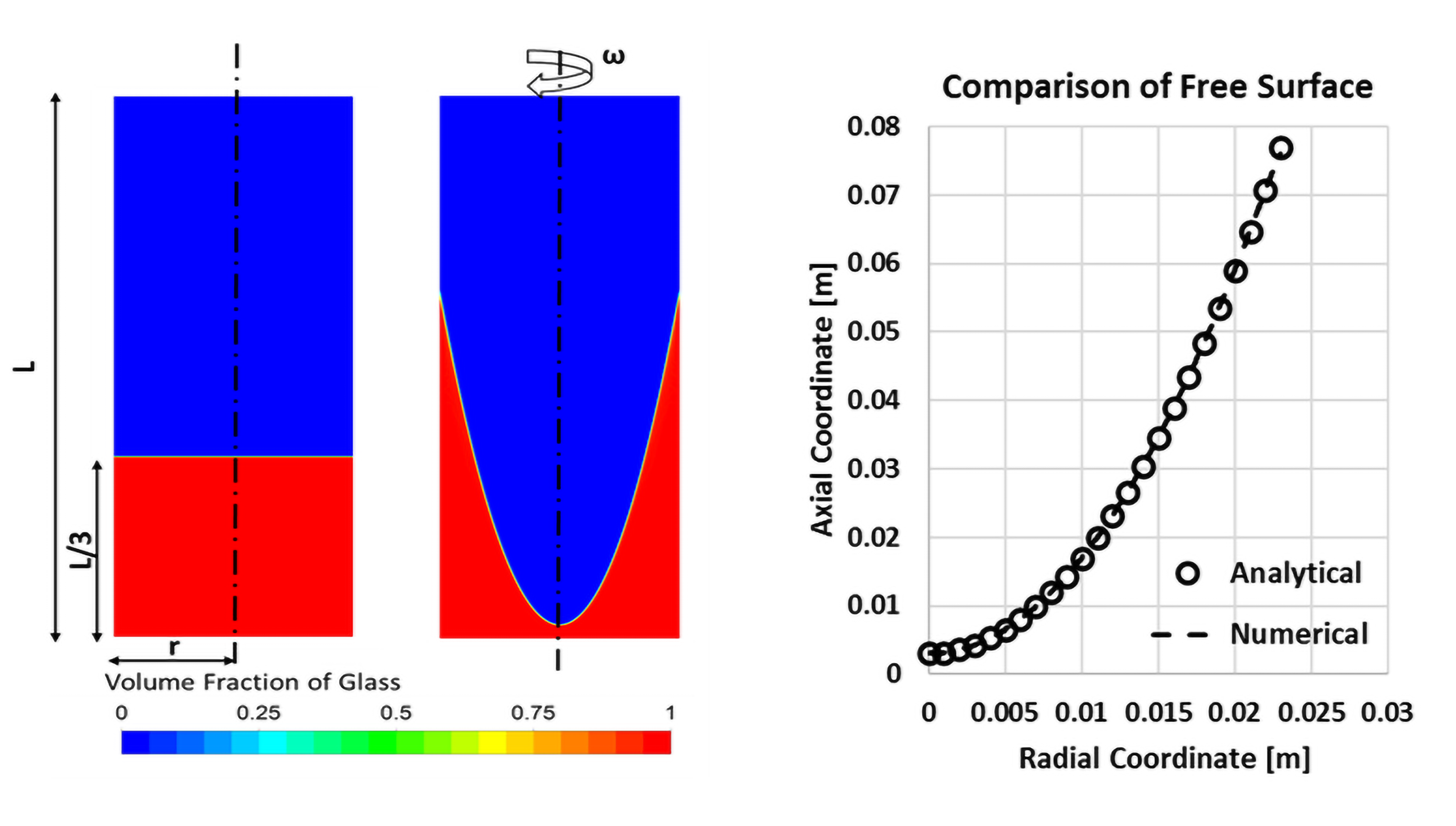
The CFD analysis is carried out using a 2D axisymmetric swirl model. The cylindrical tank has a radius of 0.023 [m] and a total height of 0.12 [m]. The computational domain consists of a quad-structured mesh of 0.2 [mm] size, with a total of 69K elements. Molten glass is patched up to the height of 0.04 [m] and the rest of the domain contains air. The pressure at the top-most point on the axis is fixed to 1 atmosphere absolute pressure. The density and viscosity of the molten glass are 2500 [kg/m^3] and 100 [kg/m-sec], respectively. The density and viscosity of the air are 0.255 [kg/m^3] and 2e-05 [kg/m-sec], respectively.

This case study contains two variants:

1. Rotating tank at 5000 [rpm] with 981 [m/sec^2] downward acceleration, resulting into a final parabolic free surface profile.
2. Rotating tank at 5000 [rpm] with 9.81 [m/sec^2] downward acceleration, resulting into a final thin film formation at the vertical rotating wall.

3.2.1. Case Study 2A: 5000 [rpm] and 981 [m/sec^2] Downward Acceleration

In this case study, the operating conditions are maintained in such a way that the free surface profile is fully parabolic within the specified domain dimensions.

For a two-phase flow in a closed rotating cylinder as shown in the Figure 5, when the bottom wall of the spinner is fully wetted by the liquid, the analytical free surface profile as a function of radial coordinate r is defined as [10]:

Where, h₀ is the initial liquid height, ω is the rotational speed, g is the downward acceleration and R is the outer most radius of the cylinder.

The analytical pressure field in the liquid for the above-mentioned condition is defined as:.

Where, ρ is the liquid density, r and z are the radial and axial coordinate, P₀ is the hydrostatic pressure at the bottom-most point on the axis corresponding to r = 0 and z = 0.

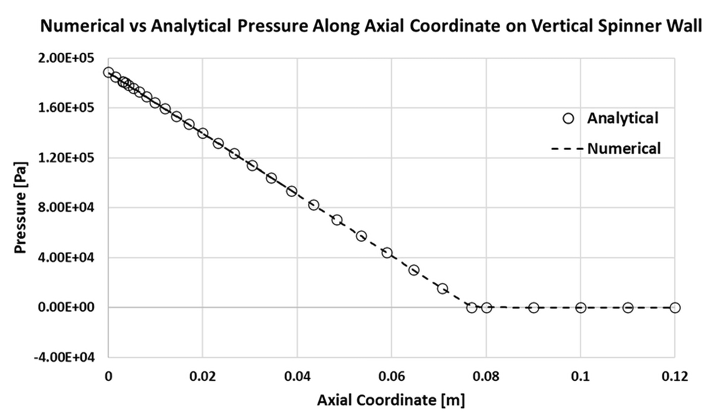
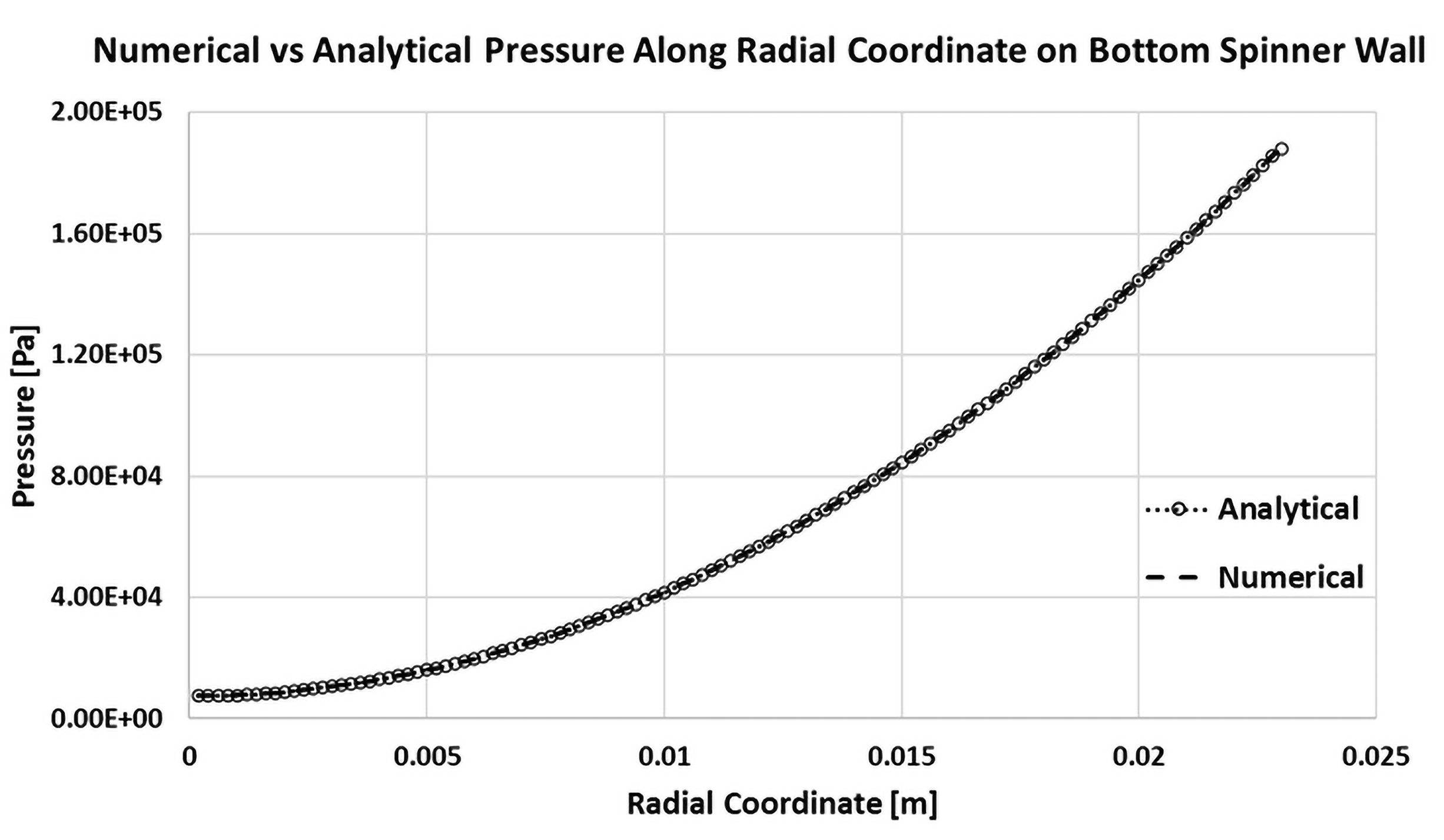
The schematic diagram of the vertical spinner is shown in the Figure 5. A perfect match is found between the CFD results and the analytical solution for the free surface shape along the bottom and the vertical spinner walls as shown in the Figure 6, whereas pressure distribution along axial and radial coordinates are shown at the Figure 7 and Figure 8 respectively.

3.2.2. Case Study 2B: 5000 [rpm] and 9.81 [m/sec^2] Downward Acceleration

In this case study, the operating conditions are maintained in such a way that the free surface profile forms a film on the vertical spinner wall.

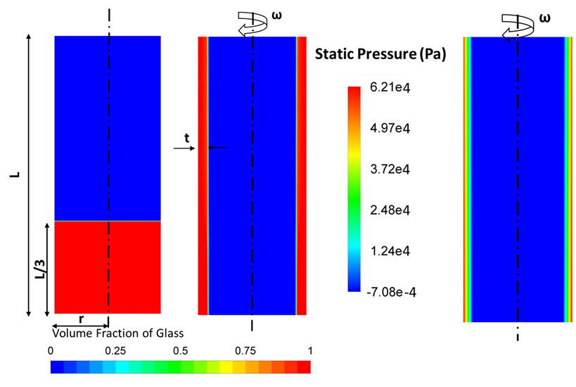
Form the conservation of mass, the final film thickness (t) as shown in the Figure 9, can be calculated as:

Where, R is the spinner wall radius, V₀ is the initial volume of glass filled, and L is the cylinder height.

The final film thickness (t) is expected to be around 4.2 [mm] using the analytical calculation. The CFD predicted film thickness is also found to be 4.2 [mm] in the final solution.

The pressure build-up at the bottom most point on the spinner wall due to rotation and hydrostatic head is analytically calculated as:

Where, ω is the rotational speed. As shown in the Figure 9, the CFD reported maximum static pressure is found to be 6.21e4 [Pa] which is very close the analytical value with an error of less than two percent.

3.3. Case Study 3: Modeling of Representative Fiberization Spinner

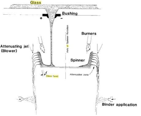
The objective of this study is to predict and validate the glass film thickness and the mass flow rate generated in the spinner outlet holes due to the rotation of the fiberization spinner. In the actual fiberization process, the glass viscosity is maintained around log3 viscosity (1000 [Poise]) by controlling the temperature. The molten glass is poured from the top as a single stream in the rotating spinner as shown in the Figure 10 [4]. Due to the high viscosity of the molten glass, there is a negligible splashing of the molten glass when the glass stream impinges on the rotating spinner. The molten glass forms a thin film on the bottom wall that creeps along the spinner walls. Finally, the molten glass is extruded into thin streams due to high centrifugal force as it passes through thousands of small orifices in the vertical section of the spinner wall.

The CFD analysis is performed on a representative geometry as shown in the Figure 11 using a 2D axisymmetric swirl model as it is sufficient to capture the required physics and to validate it against the analytical solution. The representative spinner dimensions, fluid material properties, and operating parameters are referenced from the publicly available literature [3,4,6,9]. Following engineering approximations have been made in this problem:

1. Molten glass is injected from the bottom inlet while ensuring the same mass flow rate as the primary focus of this work is on the film formation and the extrusion process.
2. Spinner holes are represented as slotted disks rather than cylindrical holes due to 2D axisymmetric modelling.
3. All the material properties and operations conditions are taken at 2000 [F] using isothermal assumption corresponding to log3 viscosity for the glass type selected in this work.

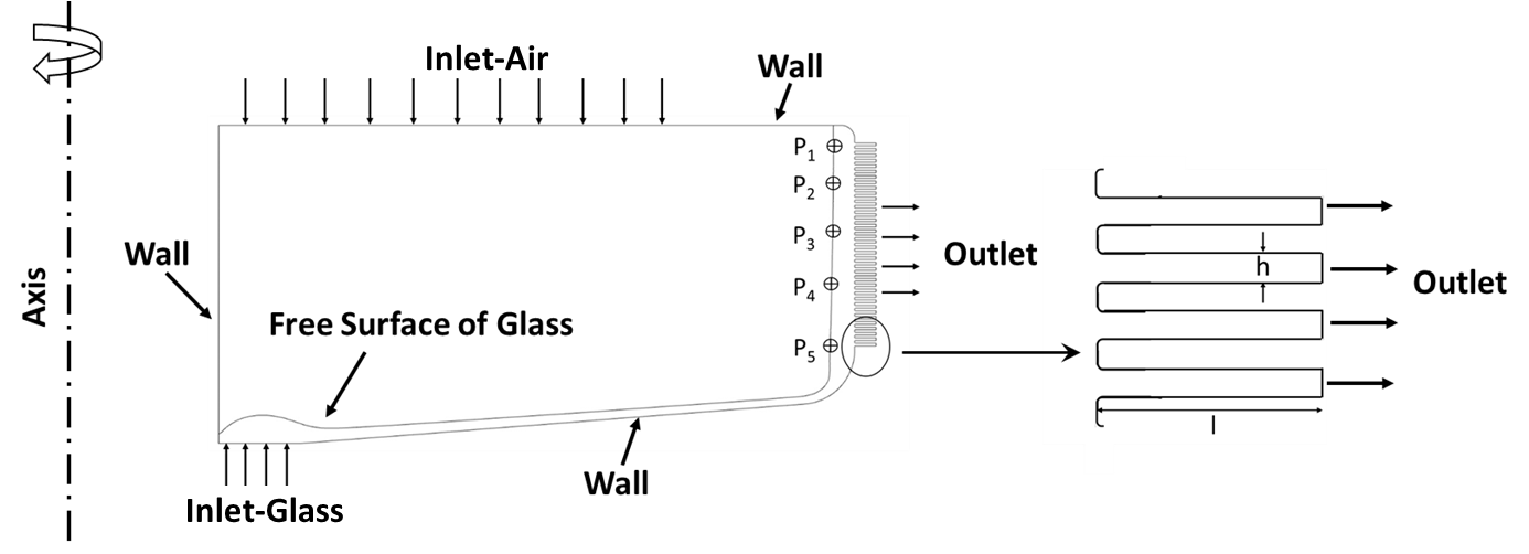
In the representative geometry as shown in Figure 11, the spinner wall outer radius is considered as 188 [mm], outlet slots have a length (l) of 3.85 [mm], and height (h) of 0.5 [mm]. The density and viscosity of the molten glass are 2500 [kg/m^3] and 100 [kg/m-sec]. The density and viscosity of the air are 0.26 [kg/m^3] and 1.8e-05 [kg/m-sec], respectively. The spinner rotation speed is 3000 [rpm], the glass flow rate is 1.07 [kg/sec] and the system is open to the atmosphere.

The CFD methodology is developed using a step by step approach by decomposing the complex problem into sub-problems:

1. In the first step, mass flow rate validation is done against the analytical solution for a single spinner 3D pipe rotating in the space about the actual spinner axis.
2. In the second step, the representative 2D axisymmetric swirl fiberization spinner model is validated using the analytical approach developed in the first step.

3.3.1. Case Study 3A: Validation of Molten Glass Flow Field in a Single Rotating 3D Pipe

The objective of this study is to predict and validate the mass flow rate generated in the single 3D rotating pipe open to the atmosphere at both ends. In this rotating pipe flow problem, the centrifugal force balances against the viscous force due to wall friction at the pipe walls as there are no external pressure gradients.

The pressure-drop in a pipe with fully developed laminar flow profile is given as [10]:

For a fully developed, laminar flow in a circular pipe, the Darcy’s friction factor f is defined as:

Where W_avg is the average flow velocity in the pipe in the relative frame, D_h is hydraulic diameter, μ is liquid viscosity, ρ is liquid density, L is pipe length, Re is Reynolds number based on the hydraulic diameter which is same as pipe diameter D.

The fluid pressure increases radially as the pressure gradient balances the centrifugal force in a rotating fluid under radial equilibrium, as shown below [10]:

The mass flow rate can be calculated by using the average relative velocity in the pipe obtained by equating equation 16 and equation 18, as shown below:

Where, ω is the rotational speed, r_i is the inlet face radial coordinate, and r_o is the outlet face radial coordinate.

The single 3D pipe having a diameter of 0.5 [mm] and a length of 8 [mm] is rotating at 3000 [rpm] about the spinner axis. The pipe inlet face has a radial coordinate (r_i) of 180 [mm] and the outer face has a radial coordinate (r_o) of 188 [mm]. The pressure drop calculation is done assuming a fully developed, laminar flow profile in the entire pipe. The entrance length is expected to be 0.6D under creeping flow condition [11]. The computational domain is a 3D cylindrical pipe having approximately 433K, hybrid elements. The pipe has a single-phase molten glass flow having a density of 2500 [kg/m^3] and a viscosity of 100 [kg/m-sec].

The analytically predicted mass flow rate is 1.74e-06 [kg/sec]. The CFD predicted mass flow rate comes as 1.72e-6 [kg/sec], which matches well with the analytical results. The small difference in results is due to the entrance length effect which is not accounted in the analytical calculations.

3.3.2. Case Study 3B: Validation of the Representative Fiberization Spinner CFD Model

The objective of this study is to predict and validate the glass film thickness and the mass flow rate generated in the spinner outlet holes due to rotation for the representative fiberization spinner. The glass film thickness is an important design parameter and at no point, the glass should spill out of the spinner. The problem schematic and model dimensions are outlined in the Figure 11.

The analytical calculation methodology developed in case 3A also applies here. The only difference is that it requires a different expression for the friction factor and the hydraulic diameter due to the axisymmetric assumption. For a plane Poiseuille, laminar flow between two infinite-depth plates, the effective Darcy’s friction factor comes out to be 96⁄Re in place of 64⁄Re [10].The Reynolds number (Re) is based on the hydraulic diameter D_h, which comes out to be two times the gap between the parallel plates [10].

After incorporating the modifications explained above, the radial coordinate, r_f at the free surface is calculated as a function of the average relative velocity, W_avg,hole,for each slotted hole, as shown below:

Where, r_o is the radial coordinate at the hole outlet, ω is the rotational speed, and D_h is 2 times the slot height h. The analytical glass film thickness is calculated as (r_o- r_f-l), where l is the length of the outlet slot, as shown in the Figure 11.

The 2D computational domain consists of 70.2K quad-pave mesh elements. The mesh is sufficiently resolved in the regions where the glass film is expected to form. There are around 8-10 elements in any narrow outlet passage. The solution methodology is adopted as described in the section 3. This simulation takes about 2-3 hours on 32 CPUs (Intel Xeon Gold 6142, 2.6 GHz).

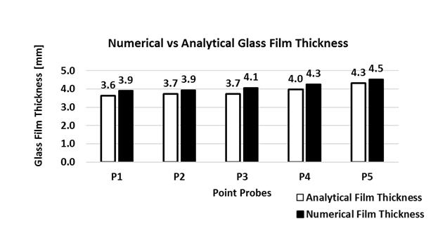
The glass thickness and the mass flow rate are measured at the five points (P1-P5), which are marked on the intersection of free surface and the radial lines passing through the centre of different holes as shown in Figure 11 For each measurement point, the CFD predicted glass film thickness is compared with the analytical calculations and both are found to be in a very close agreement as shown in the Figure 12.

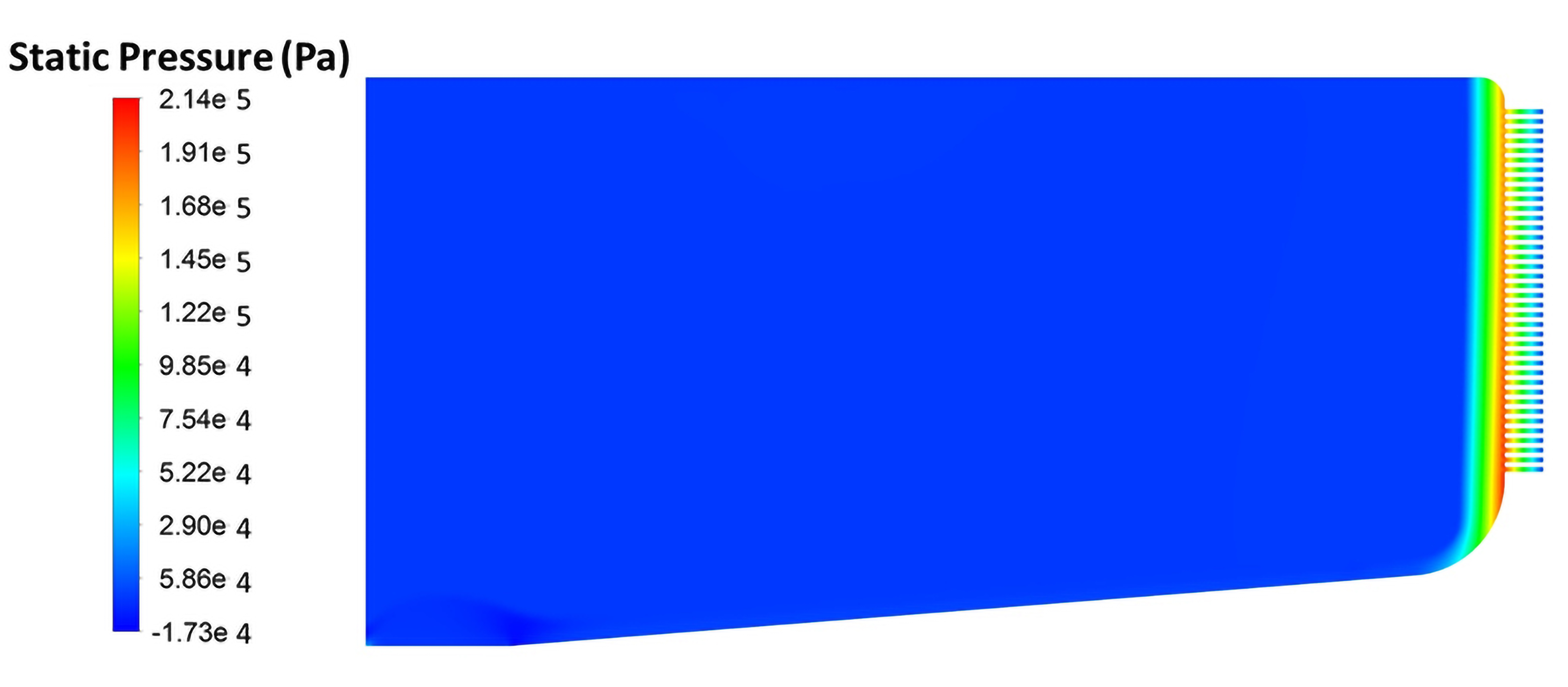
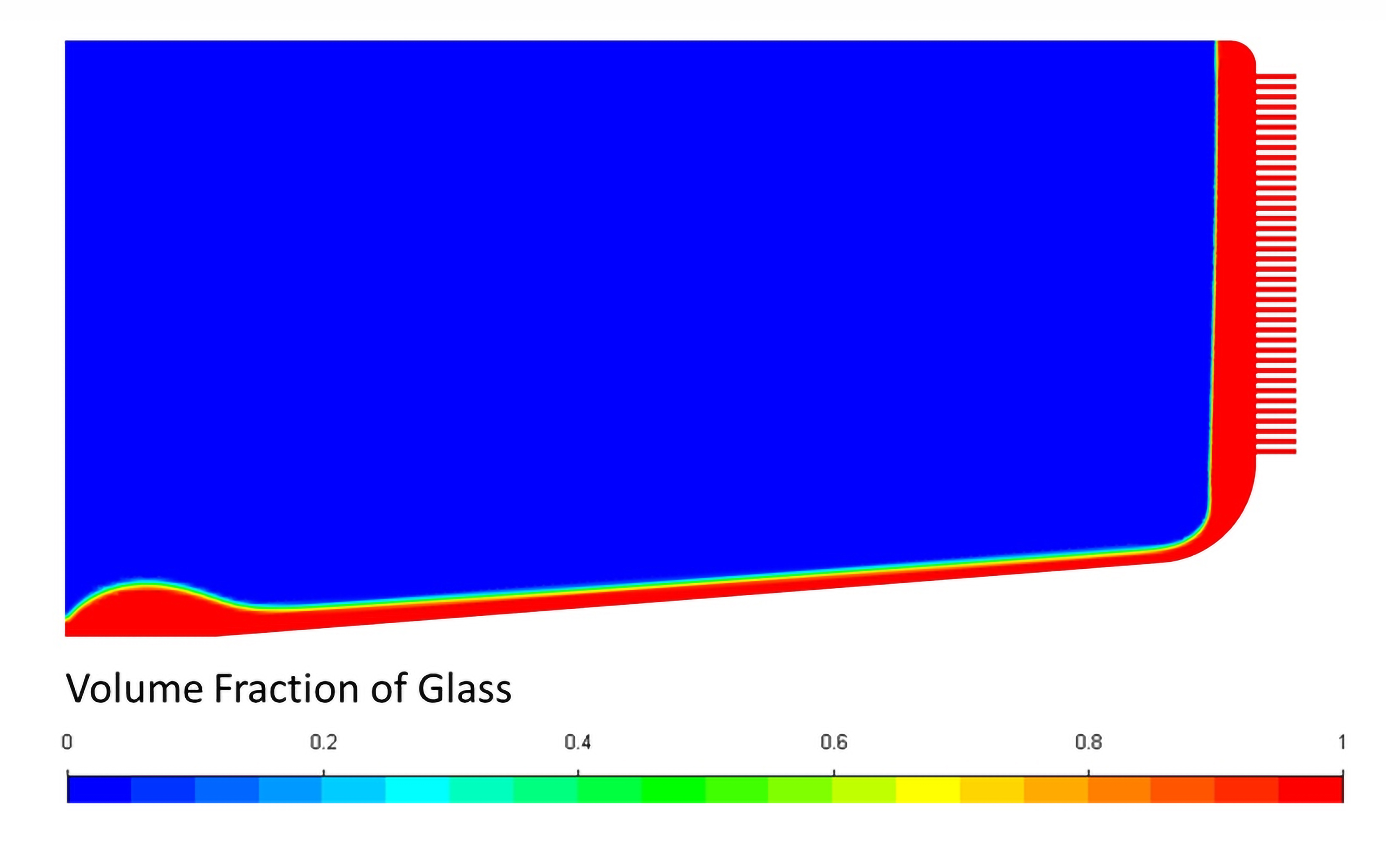
The contours of static pressure and volume fraction of glass are shown in the Figure 13 and Figure 14, respectively. It is observed that the CFD predicted maximum pressure at the rotating wall is about 2.1e5 [Pa] and the maximum glass thickness is 4.5 [mm]. The analytically calculated pressure corresponding to the maximum glass thickness comes out as 2e5 [Pa], which is very close to the CFD predicted value.

4. Conclusion

Experimental methods are very expensive, energy-intensive, and unsafe, hence the use of CFD based design and process parameter optimization is very desirable for the rotary fiberization process. Obtaining a steady-state solution for such an application involving molten glass filling, high rotation, highly viscous flow, thin glass film-forming, and extrusion through small orifices is a very challenging numerical problem.

In the present work, the complex problem associated with rotary fiberization spinner is systematically decomposed into fundamental case studies. Both the numerical and analytical methodologies are consolidated to resolve these physics accurately and efficiently. All the case studies are successfully validated for the free surface profile, glass film thickness, mass flow rate, and pressure distribution. The VOF method is able to handle the complex physics involving highly rotating, viscous flows in a robust fashion. The pseudo-transient solver along with the stabilization methods allows obtaining a significantly faster solution as compared to the traditional transient approach.

The current work focuses on the simplified analysis of the rotary glass fiberization spinner by capturing all the required physics using a representative 2D axisymmetric swirl model. However, as an extended work, the proposed CFD analysis methodology can be easily applied to an actual fiberization spinner, 3D sector model. The authors have successfully carried out a non-isothermal analysis using the proposed methodology after applying the appropriate thermal boundary conditions, but it is not presented in this work.

References

[1] F. T. Wallenberger, J. C. Watson, and H. Li, Fiber Glass, ASM Handbook, Vol. 21: Composites (#06781G), 2001.
[2] Benjamin Bizjan, Marko Peternelj, Brane Širok, Experimental investigation of melt fiberization from a perforated rotor spinning machine, Chemical Engineering Research and Design, 2015. View Article
[3] Kraševec B., Širok B., Hočevar M., Bizjan B., Multiple regression model of glass wool fibre thickness on a spinning machine. Glass Technology - European Journal of Glass Science and Technology Part A, Vol. 55, No. 4, pp. 119-12, 2014.
[4] John J. McKetta Jr, Encyclopedia of Chemical Processing and Design: Volume 21, 1984.
[5] W.Arne, N.Marheineke, A.Meister, S.Schießl, R.Wegener. Finite Volume Approach for the Instationary Cosserat Rod Model Describing the Spinning of Viscous Jets. Journal of Computational Physics, 294:20-37, 2015. View Article
[6] W.Arne, N.Marheineke, J.Schnebele, R.Wegener. Fluid-fiber-interaction in Rotational Spinning Process of Glass Wool Production. Journal of Mathematics in Industry, p. 1:2, 2011. View Article
[7] Jure Mencinger, Benjamin Bizjan, Brane Širok, Numerical simulation of ligament-growth on a spinning wheel, International Journal of Multiphase Flow, 2015. View Article
[8] Ansys Fluent Theory and User’s Guide, Release 2020R2, Ansys Inc., 2020.
[9] Raimund Wegener, Multiphysics and Multimethods Problem of Rotational Glass Fiber Melt-Spinning, International Journal of Numerical Analysis and Modeling, Series B, 2012.
[10] Yunus A Çengel, John M Cimbala, Fluid mechanics: fundamentals and applications, New York, NY: McGraw-Hill Education, 2018.
[11] Sushanta K. Mitra, Suman Chakraborty, Microfluidics and Nanofluidics Handbook, Two Volume Set, 2011.