Journal of Fluid Flow, Heat and Mass Transfer (JFFHMT)

ISSN: 2368-6111

1. Introduction

Crossflow heat exchangers are being engaged in many thermal applications, such as automotive radiator, air conditioning, refrigeration, and data center liquid cooling systems [1]–[3]. The thermal performance of an entire heating and cooling system is strongly influenced by the heat exchanger performance. Characterization of the transient behaviour of crossflow heat exchanger is of great significance in many applications, particularly, due to sudden change in their operating conditions. Evaluation of transient performance and modeling the heat exchangers at a varied mass flow rate and temperature are important because they frequently take place in real-world applications. In this study, 3D transient simulation of liquid-to-air cross flow minichannel heat exchanger (MICHX) has been carried out for a sudden change in liquid mass flow rate. This can be analogous with the thermostat operation, which regulates the operating temperature of the engine by opening and closing in response to the step-change in the coolant flow rate. Numerical simulations provide  the insight of various thermal parameters including heat transfer coefficient and Nusselt number associated with the performance of heat exchangers in transient situation. Heat exchangers are made to work under specific steady state conditions. However, due to transient behavior of heat exchanger in startup and shut down or during non-stationary function like failure, predicting of heat exchanger performance under a dynamic load or operational condition becomes  the main challenging issue [4]. Modeling and characterization of transient phenomenon has attracted the attention of many researchers for designing reliable and efficient thermal management systems. Both the mass flow and temperature variation scenarios are significant since they commonly occur in real life applications [1].

Studies predicted the impact of step variations in inlet temperature and mass flow rate of hot fluid on conventional heat exchanger performance. In 1954, Dusinberre [5] accomplished the early numerical analysis for modeling and examining the dynamic behaviours in pipes and heat exchangers. After that, Turton [6] studied the transient behaviour of the gas-to-gas crossflow heat exchanger. They described a general finite difference method for solving the transient response under several simplifications. Later on, the transient experimental characteristics of a fin-tube water-to-air crossflow heat exchanger was performed under periodic fluid inlet temperature variations by Gartner and Harrison [7]. London et al. [8] first suggested the transient effectiveness as a new term in studying the transient responses of a heat exchanger. Mathematical models were established for characterizing and forecasting the transient performance of a counter-flow heat exchanger under a step change in the hot fluid inlet temperature and mass flow rate. Myers et al. [9] presented a transient characteristics of the average outlet temperature of two fluids under a step change to the inlet temperature in a gas-to-gas crossflow heat exchanger. The step change to the inlet temperature of either the hot side or the cold side of fluid was also predicted by Romie et al. [10] using a double Laplace transform technique. Pearson et al. [11] studied dynamic response of air outlet temperature due to change in hot water mass flow rates. The authors used a commercial tube and plate-fin, serpentine, water-to-air cross flow heat exchanger in their analytical, experimental, and numerical studies. They determined the gain and time constant for the heat exchanger and tabulated the comparisons among the experimental data, numerical computer solutions, the extended form of Gartner’s model, and their derived analytical model.

Several researchers studied dynamic responses to both temperature and mass flow variations. Mishra et al. [4] Investigated dynamic performance of crossflow heat exchangers due to perturbations in hot fluid inlet temperature and both fluids mass flow rates. The authors reported that mean exit temperatures of both the fluids increased or decreased with the simultaneous increase or decrease in flow rates of the two fluids. They also observed that mean exit temperatures increased with the larger disturbance in hot fluid, while decreased with the larger disturbance in cold fluid. Silaipillayarputhur and Idem [12] performed an investigation  on transient response of a cross flow heat exchanger subjected to temperature and flow perturbations. They compared the results of the crossflow exchanger with the parallel flow and the counter flow heat exchangers. In case of the mass flow step change, authors observed the reduced thermal performance of the crossflow heat exchanger compared to the parallel flow and the counter flow arrangements. However, they noticed the enhanced thermal response time for three or more passes of the crossflow heat exchanger.  They also found the decreased tube-side pressure loss in the crossflow heat exchanger. Silaipillayarputhur and Idem [13] performed another numerical analysis of a single-pass crossflow heat exchanger to investigate its transient performance due to step change in inlet temperature and mass flow rate. They reported that the transient response of the primary fluid displayed a time lag, where outlet fluid temperature changes were not initially apparent. The time lag became gradually shorter with the increase of the step change in flow rates. In contrast, they reported the instantaneous temperature response and immediate change in outlet temperature of the secondary fluid. Gao et al. [1] numerically investigated the transient response of a 2-D unmixed–unmixed crossflow heat exchanger for variations in the inlet temperature and fluid mass flow rates. They developed mathematical models of the transient effectiveness of the crossflow heat exchanger to be useful for the selection of heat exchangers and a dynamic analysis of data center liquid cooling and hybrid cooling systems. The transient behaviour of crossflow heat exchanger was numerically studied by Mishra et al. [14] for step, ramp and exponential perturbations. It was observed that the longitudinal conduction plays an important role with the increase in NTU. Authors described the dynamic performance of the crossflow heat exchanger, the effect on the dynamic performance of longitudinal conduction and axial dispersion. Gao et al. [15] examined several experimental test on transient response under varying server powers and operating conditions on a data center cooling infrastructure facility to evaluate the transient response in a data center.

A crossflow MICHX provides several benefits over a typical conventional heat exchanger. These benefits include intensified heat transfer rate, reduced air blower capacity, minimized liquid pump power for a particular flow rate, reduced weight, and smaller unit size [16]–[18]. Kim and Bullard [19] evaluated the performance of MICHX  and finned tube condenser as a benchmark. They reported 35% reduction of refrigerant charge in the MICHX design and 35–55% reduction of core volume and weight for the identical energy efficiency ratio (EER). The performance of a unitary split system using MICHX with a conventional fin-tube outdoor coils for air conditioning and heat pumping applications were compared by Kim and Groll [20]. Authors reported that MICHX needed 23% less face area and 32% less refrigerant-side volume than that of the baseline heat exchanger.  The improvement in EER ranged from, depending on the air-side fin density and heat exchanger orientation.

Fotowat et al. [21] experimentally investigated the transient response of a MICHX with step variation of hot fluid mass flow rate. The researchers characterized the fluids outlet temperatures, response time, and residence time. However, they did not evaluate the heat transfer coefficient (HTC) and Nusselt number (Nu) when the heat exchanger is subjected to a change in the hot fluid mass flow rate.  This is because of the impracticability to experimentally measure the inner surface temperature of the 1mm channel as well as the temperature difference between liquid and wall, especially in transient situation. The numerical simulations are appropriate to practical research of fluid flow and heat transfer parameters in heat exchangers [22]. These are very useful supplement to the interpretation of the experimental data, where temperature fields and heat fluxes are very difficult or impossible to measure. The central focus of this research work is to predict the heat transfer coefficient and to develop the correlations for dimensionless temperature and Nusselt number in transient situation.

Since heat exchanger is one of the key components of energy conversion systems, research on MICHXs can be improved and extended through exploring novel schemes that exhibit more compact and enhanced heat transfer.No numerical data is available for 3D transient thermal performance and behaviour of serpentine liquid-to-air crossflow MICHX. Most of the researchers obtained simulations for simple geometries of 2D crossflow heat exchangers with some simplifying assumptions. A few numerical solutions are available for 3D transient modeling of simple pipes; however, such solutions do not represent the real-world scenarios. The complexities of heat transfer and fluid motion in a serpentine liquid-to-air crossflow MICHX make it challenging for the researchers to obtain 3D transient simulations. The findings of the literature survey unveiled the great necessity of further research on 3D transient heat transfer in the liquid-to-air crossflow MICHX. This research is achieved with the intention of filling the current information gaps as much as possible. The current research is numerically done in a liquid-to-air cross flow MICHX for perturbation in hot fluid mass flow rate. Authors have evaluated the transient heat transfer coefficient and developed correlations for transient dimensionless temperature and Nusselt number, which signifies the novelty of current research. These correlations can be useful sources for the future researchers working on MICHX as their applications become more widespread. The established models, data, and correlations can be valuable source of improving the effective efficiency and design control strategy of MICHX. It is also anticipated that the designers can utilize the transient results to develop process control strategies for heat transport devices due to a sudden change in operating conditions.

2. Numerical Methodology

2.1. Geometry Modelling

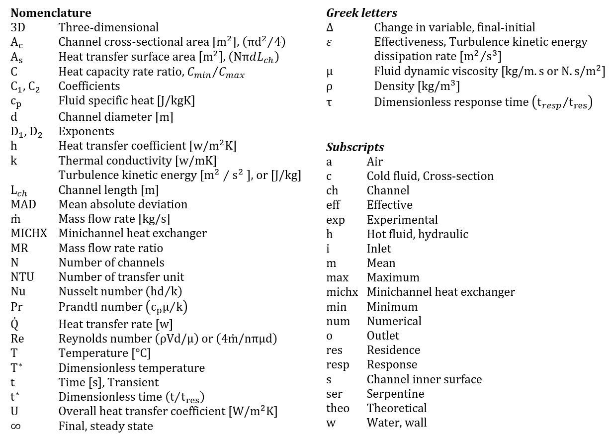
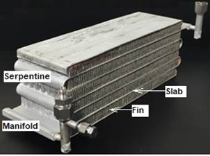
In the current research, 3D transient heat transfer simulation has been conducted in a 5-pass single-loop MICHX with the purpose evaluating transient behaviour of the heat exchanger. This is also a demonstrative representation of a real heat exchanger used by Fotowat et al. [21]. The geometric data and specifications of the device are illustrated in Table 1.

Table 1: Specifications of the device.

No. of channels/tube	68
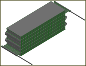
Channel diameter	1 mm
Port-to-port distance	1.463 mm
Slab width, x-direction	100 mm
Slab thickness, y-direction	2 mm
Slab length, z-direction	305 mm
Fin density per 25.4 mm	12
Fin height	16 mm
Fin thickness	0.1 mm
Inlet & exit tube diameter	4.76 mm

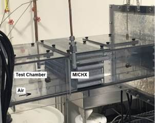
The photograph of the physical device (MICHX) used in this study, CAD model, and the dimensions of the slab and minichannels are shown in Figures 1(a), 1(b), and 1(c) respectively.

(a) (b) (c)

2.2. Computational Domain

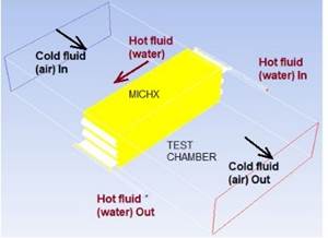
The computational domains have been selected in consideration of the test chambers incorporating minichannel heat exchanger (MICHX) as used by Fotowat et al. [21] in their experimental study. The computational domain consists of a minichannel heat exchanger (MICHX) and a test chamber in a liquid-to-air cross flow orientation. These are equipped in the experimental setup of Thermal Management Research Laboratory at University of Windsor. The domain includes two continuums and the solid heat exchanger. Hot fluid (water) flows through the channels inside the MICHX, while the cold fluid (air) flows through the test chamber in a cross-flow orientation as presented below.

(a) (b)

In Fig. 2(a), the MICHX and the test chamber are shown without insulation. However, in the experiment, all these regions were fully insulated. In Fig. 2(b), the white color represents the parts that are insulated. The top and bottom of the MICHX are also white, but invisible due to yellow colored MICHX core. Heat transfer takes place between hot and cold fluids via solid slabs and fins.

2.3. Mesh / Grid Generation

The domain consists of two major components, a minichannel heat exchanger (MICHX) and a test chamber. The MICHX consists of two  manifolds, five core-slabs with sixty eight minichannels, two dummy- slabs,  four serpentine bends, and eight hundred and forty six fins. Meshing of each component is discussed in this section. Various meshing approaches have been used to generate appropriate grids for each component in the computational domain. GAMBIT is used to create geometry and generate mesh applicable for CFD simulations using ANSYS FLUENT. The geometry contains millions of surfaces and volumes because of the complex shape of the models. Due to the complexity of the geometry, it is impossible to generate a single structured mesh for the whole domain. The model is, therefore, divided into several sub-sections including air (test chamber), manifolds, serpentines, channels, and solid slabs and fins. A computer with 16 parallel processors and 128GB random access memory (RAM) is used for this current study. Structured hexahedral meshes are generated for the fins. Cooper hexahedral and wedge meshes are generated for the serpentine bends and channels, while unstructured tetrahedral, hybrid and wedge meshes are created for the rest of the model. Some of the channel and air meshes are shown in Figures 3(a) and 3(b).

(a) (b)

2.4. Assumptions

In the current study, the inlet air temperature of  is heated by the inlet water temperature of  for all cases. The relative humidity (RH) of air at inlet condition is in the range of 15% to 40%. At 1 atm pressure, the maximum moisture content of the inlet air at 40% RH is about 4g/kg dry air. Since air is heated by hot water, the moisture content of outlet air (at  max.) would be similar to that of the inlet air. In this situation, heat transfer contribution of the water vapor content in the air is assumed to be negligible ( deviation) within the working conditions.

In the current study, the bulk temperature of air varies from to . Compared to the properties of air at the standard temperature of 20℃, the maximum deviation of density, specific heat, viscosity, and conductivity of air are computed 2.4%, 0.02%, 1.90%, and 2.11%, respectively. In order to reduce the computational complicacies in the current 3D transient heat transfer simulation, the constant thermophysical properties of air at standard temperature of 20℃ and pressure of 1 atm [NIST] are used.

• fluids are single phase incompressible Newtonian
• thermophysical properties of liquid are the functions of temperature but independent of pressure
• change in thermophysical properties of air and solid (aluminium) within the working temperature are negligible
• heat transfer takes place between liquid and air only
• walls of serpentine and manifolds are adiabatic
• no radiation heat transfer in the system
• no heat loss or gain to or from the surroundings

2.5. Governing Equations

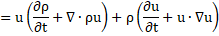
In the current study, the Reynolds-averaged Navier-Stokes (RANS) equations have been solved by using ANSYS FLUENT, a finite volume method (FVM) based CFD software. Based on the key assumptions, these [23] are illustrated below

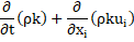
Continuity or mass conservation:

Momentum conservation:

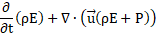
Energy conservation:

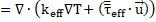
where, the effective thermal conductivity,  and the deviatoric stress tensor,

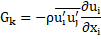
Turbulence kinetic energy, k:

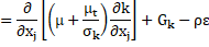
where, the term,  for the transport of k is,

Turbulence energy dissipation, ε:

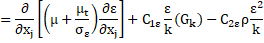
where, , and are constants, and  is the turbulent Prandtl number for .

2.6. Grid Independency Study

It is essential to note that the mesh fineness plays a vital role in the computational fluid dynamics (CFD) simulations. In the CFD, the simulation time, cost and accuracy greatly depend on proper mesh generation in the computational domain. In order to establish the accuracy and consistency of the numerical results, and to retain the computational cost low, the grid independency test has been performed in the current study. Several grid systems have been used to check grid independency by solving the Navier-Stokes governing equations. The initial computational domain consists of 5.8 million of cells. If the fine grid is doubled to the coarse one in the whole domain then the total volume of meshes goes very high and the computer become frozen. As a result, grids are adapted gradually near the wall, especially for the heat exchanger core where heat transfer takes place between the hot and cold fluids. These are presented in Figure 4.

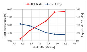
The relative deviations in the heat transfer rates () and the pressure drops () in two consecutive grid systems (GS) are computed. The variations of  between GS1 & GS2, GS2 & GS3, GS3 & GS4, and GS4 & GS5 are found 13.0%, 12.7%, 11.0%, and 0.5%, respectively. While the respective variations of  between GS1 & GS2, GS2 & GS3, GS3 & GS4, and GS4 & GS5 are observed 4.1%, 14.4%, 4.2%, and 0.8%. The grid system of the numerical simulations has been chosen when the maximum variations in both the  and the  in two successive GS are observed about 1%. The selected GS of the model in the current study contains 7.85M of cells.

2.8. Computational and Physical Setup

In the current study, the CFD has been carried out in 3DDP, pressure-based, absolute velocity formulation and implicit scheme to solve the flow and heat transfer problem in the liquid-to-air crossflow MICHX. Details of the physical and computational fundamental parameters are described in this section.

Model selection:

A turbulence model is used to capture the turbulence parameters developed in the heat exchanger. This model is chosen due to the high Reynolds number of the fluids at the inlet and the outlet boundaries as well as three-dimensional unsteady random fluid motion at headers, manifolds, and heat exchanger core. Preliminary simulations have been conducted using Standard - and Shear Stress Transport (SST) - turbulence models. Numerical predictions have been compared to the experimentally measured data. The Standard - with EWT shows better results than the others. As a result, Standard - turbulence model is used in the current study. Viscous heating is enabled to capture the effects of viscous heating on the thermal performance of the heat exchanger.

Properties of materials:

The thermophysical properties, such as density, specific heat, viscosity and thermal conductivity of a fluid signify the response of the fluid due to the variation in its speed or flow rate, temperature or combination of both. In the current study, the all working fluids have been assumed as incompressible within the operating temperature and flow regime. The transport properties of the hot fluid (water) have been considered temperature dependent. While the properties of air and solid (aluminum) have been assumed independent of temperature.

Initial and Boundary conditions:

Following boundary conditions are applied in the current study:

• Inlet liquid: Temperature and mass flow rates are specified
• Inlet air: Temperature and mass flow rate or velocity are specified
• Outlet liquid: Pressure outlet boundary condition is specified.
• Outlet air: Pressure outlet boundary condition is specified
• Headers, manifolds and serpentines: Zero heat flux is specified.
• Walls: No slip, stationary wall and zero heat flux or adiabatic thermal boundary conditions are specified

3. Data Processing

3.1. Heat Transfer Performance Parameters

Following fundamental equations have been used for computations of convective heat transfer:

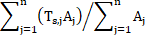
Heat transfer rate (

Heat transfer coefficient

3.2. Mass Flow Rate Ratio (MR)

The mass rate ratio (MR) is defined as the ratio of the new hot fluid inlet mass flow rate after step change (over the initial hot fluid inlet mass flow rate . It is calculated as

3.3. Residence Time()

Residence time () is defined as the time occupied by the hot fluid to travel the heat exchanger core, where heat transfer takes place between the hot fluid and the cold fluid. It is computed as

3.4. Dimensionless Parameters

In order to generalize and conveniently report the simulation outcomes, parameters have been non-dimensionalized.

Convective heat transfer relationship [24]:

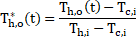
Transient dimensionless outlet temperature:

Dimensionless time (t*):

The residence time  is the time () employed by the hot fluid to pass through channel, where heat exchanges between the hot and cold fluids.

Dimensionless response time ():

The response time () is defined as the time required for a fluid to reach from one steady state to another final steady state situation.

4. Model Verification and Validation

In order to ensure that the numerical results of the computational model are accurate and consistent, model verification and validation have been accomplished. These are illustrated in this section.

4.1. Model Verification

The roundoff error, the iterative convergence error, and the discretization error have been evaluated as prescribed by AIAA (1998) [25]. With the aim of minimizing the roundoff error, CFD simulation results have been obtained using a double precision machine with 16 significant digits. In order to quantify the iterative convergence error, the effects of residuals on mass flow rate and pressure drop have been investigated. The discretization error is computed by mesh refinement. A grid independency study has been carried out to attain a high-quality CFD simulation result. Another verification has been performed by checking overall mass flow rates of both fluids and heat transfer rate of the system.

4.2. Model Validation

The transient response of a liquid-to-air crossflow heat exchanger under changes in the hot water mass flow rate has numerically been studied. Different mass flow rate ratio (MR) starting from an original value of  to the subsequent  of 0.5, 0.8, 1.5, 2.0, 2.5 and 3.0 have been solved. The hot fluid (water) inlet temperature of  and cold fluid (air) inlet temperature of  and velocity of  have been kept constant throughout all the simulations for all the mass flow steps.

With the purpose of making sure that the model precisely represents the actual applications, a set of results from transient simulations has been validated with available experimental transient data [21]. In both, the simulation and the experiment, hot fluid (water) is cooled by cold fluid (air) Figures 5(a) to 5(d) present the comparison of numerical and experimental results for the transient outlet temperature of the hot fluid due to the step change in same fluid mass flow rate. In the hot fluid outlet temperature, the numerical predictions display maximum deviation of 13.56% and mean absolute deviation (MAD) of 8.78%.  In Figure 5(e), outlet temperature of the hot fluid at quasi-steady state under various mass flow steps is summarized. At steady state, The maximum error of 8.55% and mean absolute error of 7.07% is found in the numrical results for hot fluid outlet temperature. Numerical results show good agreement with the experimental data.

(a) (b) (c) (d) (e)

Stepping up () and stepping down () of hot fluid mass flow rate perform two distinct heat transfer behaviors. The  displays a higher heat transfer coefficient while a lower heat transfer coefficient compared to the initial value of  With the referencing of , the current study overestimated (further away from the baseline or initial) the experimental data. Numerical predictions are consistent for both  and .

The numerical and experimental results for the temporal variation of cold fluid outlet temperature due to the mass flow steps have also been compared and presented in Figures 6(a) to 6(c).  In the cold fluid outlet temperature, the simulation results display maximum deviation of 12.21% and mean absolute deviation (MAD) of 9.87%.The Figure 6(d) shows the  summary of cold fluid outlet temperature at quasi-steady situation under different mass flow steps. At steady state, the maximum error of 9.74% and mean absolute error of 7.08% are found in simulations for the cold fluid outlet temperature, which are within the acceptable range of error.

(a) (b) (c) (d)

The numerical prediction of heat transfer rate at the final stedy state condition for different mass flow rate ratio (MR) also compared with the experimental results and presented in Figure 7(a).  The error in numerical predictions of the final steady-state hot fluid outlet temperature (), cold fluid outlet temperature (), and heat transfer rate () are summerized in Figure 7(b). The maximun error of 8.55% in , 9.74% in , and 8.67% in  are observed among all cases. These are within the acceptable range of error.

(a) (b)

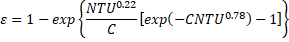
The model is also validated with the theoretical correlation. The numerical results of the final steady-state effectiveness () are compared with the theoretical steady-state -NTU correlation for the unmixed-unmixed cross flow  heat exchanger developed by Kays and London [26] .

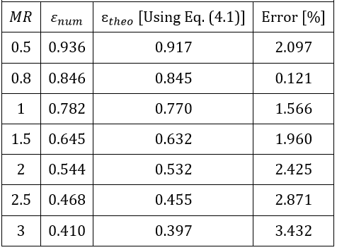
The numerical predictions and the calculated results using Eq. 4.1 are presented below in Table 2. From the results presented in Table 2, the maximum error of 3.43% is observed in numerical predictions, which shows a good agreement with the theoretical correlation. The verification and validation of numerical results ensure the reliability of the results and one can certainly depend on the accuracy and consistency of the CFD models of the current study.

Table 2. Validation with theoretical correlation [26].

5. Results and Discussions

5.1. Effect of MR on Hot Fluid Residence Time

The transient effect of hot fluid (water) MR on the residence time () is shown in Figure 8.

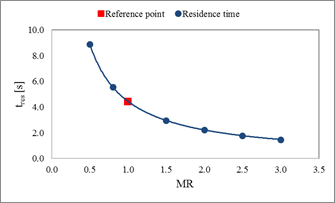
In the figure, the x-axis value of  represents the initial mass flow rate of hot fluid from which step changes are taken place. Stepping up (fold-increase) and stepping down (fold-decrease) of the hot fluid mass flow rate are  denoted by  and , respectively. It is observed that the residence time decreases with increase of mass flow step variation in a nonlinear pattern of geometric sequence. The gradient of the residence time is greater for step down scenarios than the step-up scenarios, and approaches toward the smaller magnitude. The residence time becomes double for half-fold decrease and turns into half for 2-fold increase of mass flow rate. This is because the smaller the step ratio, the lower the fluid velocity and Reynolds number of the fluid.

5.2. Transient Effect of MR on Response Time

The response time is defined as the time required for a fluid to reach from one steady state to another. In reality, the starting or initial time of transition of two fluids are not the same. There is a time delay to response of one fluid compared to the other fluid. The effects of hot fluid mass flow rate step variations (MR) on the transient response time for fold-increase and fold-decrease are shown in Figures 9(a) - 9(d). In order to compare the effects of MR on a consistent basis, the response time () is  made dimensionless by dividing it by the residence time () for the step change in hot fluid mass flow rate.

Figures 9(a) and 9(b) represent the effects of MR on the dimensionless response time () for stepping up and stepping down situations, respectively. It is clearly apparent from the figures that the response time is shorter for greater , while it is longer for smaller . The gradient is steeper for  compared to the gradient for . The response time is quantified in absolute time unit and presented in Figures 9(c) and 9(d).  The numerical prediction shows that the response time taken by the MICHX is about 30s for 2-fold increase and 110s for half-fold decrease of mass flow rate. This is because the fluid transportation velocity, molecular movement and the heat transfer coefficient increase with the increase of the mass flow rate.

(a) (b)

5.3. Effects of MR on Outlet Temperatures of Fluids

The transient variations of hot (water) and cold (air) fluids outlet temperature due to step changes in hot fluid mass flow rate are presented in Figures 10(a) and 10(b), respectively. The hot fluid mass flow rate step ratio,  defines the original or reference value. For both the hot fluid and the cold fluid, the time occupied to approach the steady state decreases with the increase of  value. At higher  value, greater steady state (final) outlet temperature is observed for both the fluids. This is because the working condition of the heat exchanger is “heats the cold fluid”. Numerical prediction shows that the higher the mass flow rate, the higher the Reynolds number and the heat transfer coefficient. The trend for transient and quasi-steady state outlet temperatures are not symmetrical for step up and step-down mass flow variations. This can be interpreted as the time dependent outlet temperatures of both the hot fluid and the cold fluid for 2-fold step up () and half-fold step down () are asymmetrical. For 2-fold step up mass flow rate, the outlet temperature of the hot fluid and the cold fluids at steady state condition are increased by 42% and 20%, respectively. Whereas, the corresponding outlet temperature are decreased by 36% and 21% for half-fold step down mass flow rate.

(a) (b)

5.4. Transient Effect of MR on the Hot Fluid and the Channel Inner Surface Temperatures

The transient variations of hot fluid and channel inner surface temperatures under hot fluid mass flow steps are presented in Figures 11(a) and 11(b), respectively.

(a) (b)

The mass-weighted average temperature of the hot fluid is computed as

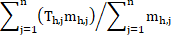
where,  denotes the temperature of the hot fluid associated with a cell in the domain and  represents the mass of the hot fluid associated with the cell.

The area-weighted average temperature of channel inner surface is computed as

where,  is the channel inner surface temperature associated with a cell in the domain and  is the facet (surface) area associated with the cell.

5.5. Correlation for Transient Dimensionless Outlet Temperature of the Hot Fluid

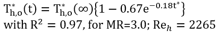
Figure 12(a) shows the variations of the dimensionless hot fluid temporal outlet temperature to the quasi-steady outlet temperature at various dimensionless time and hot fluid mass flow steps.  It is shown in the figure that at transient region, hot fluid outlet temperatures are influenced by both the time and the mass flow rate. They approach asymptotic value of 1 in the quasi-steady state. The effect of mass flow step variations on transient response of temperatures is stronger at the beginning and becomes gradually weaker with decreasing gradient.  

(a) (b)

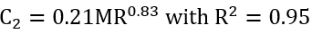
A general correlation for  in terms of  under various mass flow steps is developed. First, the correlation for  with regard to the  is obtained and presented in Figure 12(b). Expectedly, the   increases with the increase of . The variations follow a power relationship with positive exponent as

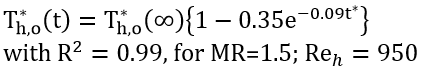
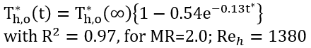
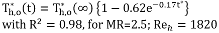
Then, the correlation for each MR is obtained and presented in Figures 13(a) to 13(d).

(a) (b) (c) (d)

The correlations for the  with regard to  corresponding to each MR are presented below:

The above relations from (5.5.2) to (5.5.5) have been correlated to obtain a generalized correlation for the  as a function of , and . These Equations can be expressed in the following form:

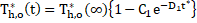
where, , as shown before in Equation (5.5.1).

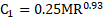
where, ,  and  are dependent on the mass flow steps. The regression analyses have been done with the purpose of obtaining  and .

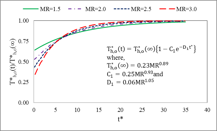
The developed generalized correlation (5.5.6) for transient dimensionless temperature of the hot fluid is compared with the numerical data for each mass flow step variations. This correlation fits all data in the transient schemes with maximum deviation of 10.39% as shown in Figure 14.

5.6. Transient Effect of MR on Heat Transfer Rate

The transient effects of step change in hot fluid mass flow rate on the heat transfer rate are shown in Figures 15(a) and 15(b). The figures present the heat transfer rate for stepping up or fold-increase scenarios. As fold-increases, heat transfer rate in the hot fluid-side, as shown in Figure 15(a), starts from a higher magnitude. On the other hand, the start-up magnitude of heat transfer in cold fluid-side, as shown in Figure 15(b), is constant for all steps. This is because of the fact that the steps have been obtained in hot fluid mass flow rate from a reference steady state condition. It can be interpreted as cooling and heating modes in the heat transfer based fluid flow.

(a) (b)

The heat transfer rate in the hot fluid drops down and cold fluid rises up from their start-up values until it reaches to the thermal equilibrium condition and becomes steady state.  For both the hot fluid and the cold fluid, increasing mass flow steps results faster and higher heat transfer rate. For any particular step, the response time is larger for the hot fluid than the cold fluid. This is because of the fact that that the hot fluid residence time is greater than the cold fluid. Another reason is that the step change has been attained in the hot fluid-side.

5.7. Transient Effect of MR on the Heat Transfer Coefficient of Hot Fluid

The transient effects of hot fluid MR on hot fluid’s heat transfer coefficient fluid is illustrated in Figures 16(a) and 16(b) below. The Figure 16(a) represents stepping up, while Figure 16(b) represents stepping down situations. The transient response of the liquid-to-air crossflow heat exchanger has been considered for mass flow steps of 0.5, 0.8, 1.5, 2.0, 2.5 and 3.0. At the start-up, it is seen that the heat transfer coefficient of the hot fluid () for fold-increase ( 1.5, 2.0, 2.5 and 3.0) is higher than that of the original value. However, the  is lower than the original value for fold-decrease ( 0.08 and 0.05). This is because of the fact that the fluid mass flow rate dictates the Reynolds number, which strongly influences the heat transfer coefficient. It is well mentioned that the steps have been obtained from a steady state condition of the original  of .

(a) (b)

ang=EN-US style='font-family:"Cambria","serif";color:black'> 

The heat transfer coefficient gradually decreases with time for stepping up, becomes constant at the fully developed region and reaches a steady state. On the other hand, the heat transfer coefficient gradually increases with time for stepping down and becomes constant at steady state.

The heat transfer coefficient of hot fluid at quasi-steady state under perturbation of the hot fluid mass flow rate is illustrated in Figure 17(a). Increasing heat transfer coefficient is found with the increase of . This is because of the fact that the higher  causes the higher temperature gradient between the wall surface and the fluid, which results in higher heat transfer coefficient.

(a) (b)

A relative heat transfer coefficient of hot fluid due a 2-fold increase and a half-fold decrease of MR is shown in Figure 17(b). Asymmetric  have been predicted for stepping up and stepping down situations. This is because of the fact that the formation of thermal and hydrodynamic boundary layers in heat transfer based fluid flow is different due to affected fluid density and hence the Prandtl number [24].

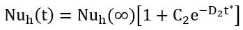
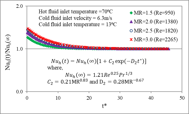
5.8. Correlation for Transient Nu at Various Re under MR

Figure 18(a) illustrates the hot fluid transient Nusselt number,  to quasi-steady Nusselt number,  with dimensionless time, and hot fluid MR.  The figure shows that at transient state, the ratio of  to   is influenced by both the time and the mass flow rate. The value of  approaches to asymptotic value of 1 in the quasi-steady state. The effect of mass flow steps on transient responses of Nu is initially stronger with higher gradient. The effect gradually reduces with smaller gradient and approaches to the quasi-steady state.

(a) (b)

A general correlation for  in terms of  at mass flow step variations is developed. The correlation for  is obtained from the best curve fit as illustrated in Figure 18(b). It is obvious from the figure that the   increases with the increase of , which is subjected to .  The variation of  with regard to  and  follows the power-law relationship with positive exponent as

for  and

                                                                                                                    

The correlation of  for each  is attained and presented in Figures 19(a) to 19(d).

(a) (b) (c) (d)

The correlations for the  in terms of  and  corresponding to each mass flow step are stated below:

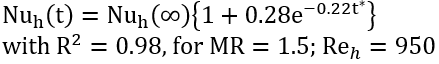
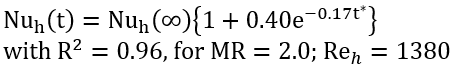
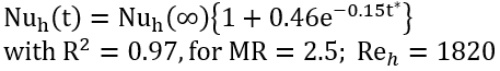
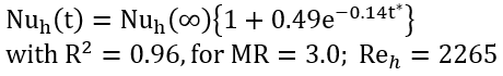
The above Equations from (5.8.2) to (5.8.5) have been< correlated to develop a generalized correlation for the as a function of ,  and . These can be illustrated in the following generalized form:

where, , derived earlier, [see Eq. (5.8.1)] for  and .

The coefficient  and exponent , both depend on the mass flow steps. A regression analysis has been carried out with the aim of attaining  and . The developed correlation (5.8.6) for transient Nusselt number of the hot fluid is compared with the numerical data for each mass flow step.  This generalized correlation fits all data in the transient schemes within 4.7% deviation as shown in Figure 20.

6. Conclusion

Numerical investigations have been conducted in a liquid-to-air crossflow minichannel heat exchanger (MICHX) subjected to mass flow step variations of 0.5, 0.8, 1.5, 2.0, 2.5 and 3.0 in hot fluid mass flow rates. Numerical simulation is the appropriate counterpart to the interpretation of the experimental measurement, where thermal and flow fields are very challenging or unfeasible to measure. In the current study, a three-dimensional transient CFD simulations have been performed in the unmixed-unmixed serpentine MICHX using ANSYS FLUENT. The hot fluid inlet mass flow rate has been varied while the other parameters for both the hot fluid and the cold fluid have been kept constant. The performance of the MICHX in terms of fluid outlet temperature, response time, and convective heat transfer has been predicted. The transient heat transfer coefficient was evaluated and new correlations for dimensionless temperature and Nusselt number in transient situations were established, displaying the uniqueness of the current study. The key findings of the current study are summarized below:

• The exit temperature of the fluid does not respond instantaneously to the variation in the hot fluid mass flow rate due to the propagation delay.
• The higher the mass flow step ratio, the higher the Reynolds number, which consequences in a longer response time for the hot fluid to be steady.
• An asymmetric trend of temperatures and heat transfers with respect to response time for the decremental and incremental step variations has been observed.
• For both the hot fluid and the cold fluid, increasing mass flow steps, results in a faster and higher heat transfer rate.
• For any particular mass flow step, the response time is larger for the hot fluid than the cold fluid due to the fact that the hot fluid residence time is greater than the cold fluid.
• For the hot fluid Reynolds number of  , the convective heat transfer coefficient of hot fluid (water) is predicted from 4084. 

• New correlations for the dimensionless transient outlet temperature of hot fluid in the form of  and the  transient Nusselt number of hot fluid in the form of  are developed.  These can serve future scientists for heat exchanger designs specifically in transient situations due to fluid mass flow step variations in crossflow MICHX, as their applications become more extensive.

Acknowledgements

Authors are pleased to express thanks to the Natural Sciences and Engineering Research Council of Canada (NSERC) for providing discovery grant (DG) to conduct the current study. The authors also thankfully acknowledge the department of Mechanical, Automotive, and Materials Engineering (MAME) at the University of Windsor for providing the opportunity of Postdoctoral research for current and continuing research.

References

[1] T. Gao, J. Geer, and B. Sammakia, “Review and analysis of cross flow heat exchanger transient modeling for flow rate and temperature variations,” J. Therm. Sci. Eng. Appl., vol. 7, no. 4, pp. 041017, 1–10, 2015, doi: 10.1115/1.4031222.
[2] M. Ismail, A. Fartaj, and M. Karimi, “Numerical investigation on heat transfer and fluid flow behaviors of viscous fluids in a minichannel heat exchanger,” Numer. Heat Transf. Part A Appl., vol. 64, no. 1, pp. 1–29, 2013, doi: 10.1080/10407782.2013.773803.
[3] M. Dehghandokht, M. G. Khan, A. Fartaj, and S. Sanaye, “Numerical study of fluid flow and heat transfer in a multi-port serpentine meso-channel heat exchanger,” Appl. Therm. Eng., vol. 31, no. 10, pp. 1588–1599, 2011, doi: 10.1016/j.applthermaleng.2011.01.035.
[4] M. Mishra, P. K. Das, and S. Sarangi, “Transient behaviour of crossflow heat exchangers due to perturbations in temperature and flow,” Int. J. Heat Mass Transf., vol. 49, no. 5–6, pp. 1083–1089, 2006, doi: 10.1016/j.ijheatmasstransfer.2005.09.003.
[5] G. M. Dusinberre, “Numerical methods for transient heat flow,” Trans. ASME, vol. 67, no. 8, pp. 703–712, 1945.
[6] J. S. Turton, “A method of evaluating transient response of gas-to-gas heat exchangers,” J. Mech. Eng. Sci., vol. 2, no. 4, pp. 349–358, 1960.
[7] J. R. Gartner and H. L. Harrison, “Dynamics characteristics of water to air cross-flow heat exchanger,” ASHRAE Trans., vol. 71, pp. 212–224, 1965.
[8] A. L. London, R. M. Cima, and A. J. Oberg, “The transient response of a two-fluid counter flow heat exchanger, the gas-turbine regenerator,” Trans. Amer. Soc. Mech. Eng., vol. 80, pp. 1169–1179, 1957.
[9] G. E. Myers, J. W. Mitchell, and R. F. Norman, “The transient response of crossflow heat exchangers, evaporators, and condensers,” J. Heat Transfer, no. February, pp. 75–80, 1967.
[10] F. E. Romie, “Transient response of gas-to-gas crossflow heat exchangers with neither gas mixed,” J. Heat Transfer, vol. 105, no. August, pp. 563–570, 1983, doi: 10.1115/1.3245622.
[11] J. T. Pearson, R. G. Leonard, and R. D. McCutchan, “Gain and time constant for finned serpentine crossflow heat exchangers.pdf,” ASHRAE Trans., vol. 80, no. 11, pp. 255–267, 1974.
[12] K. Silaipillayarputhur and S. A. Idem, “Transient response of a cross flow heat exchanger subjected to temperature and flow perturbations,” in The ASME 2015 International Mechanical Engineering Congress and Exposition, IMECE2015, 2015, pp. 1–10.
[13] K. Silaipillayarputhur and S. A. Idem, “Step response of a single-pass crossflow heat exchanger with variable inlet temperatures and mass flow rates,” J. Therm. Sci. Eng. Appl., vol. 4, pp. 044501, 1–6, 2012, doi: 10.1115/1.4007206.
[14] M. Mishra, P. K. Das, and S. Sarangi, “Transient behavior of crossflow heat exchangers with longitudinal conduction and axial dispersion,” J. Heat Transfer, vol. 126, no. June, pp. 425–433, 2004, doi: 10.1115/1.1738422.
[15] T. Gao, B. Sammakia, and J. Geer, “Dynamic response and control analysis of cross flow heat exchangers under variable temperature and flow rate conditions,” Int. J. Heat Mass Transf., vol. 81, pp. 542–553, 2015, doi: 10.1016/j.ijheatmasstransfer.2014.10.046.
[16] M. A. Hossain, Y. Onaka, and A. Miyara, “Experimental study on condensation heat transfer and pressure drop in horizontal smooth tube for R1234ze(E), R32 and R410A,” Int. J. Refrig., vol. 35, no. 4, pp. 927–938, 2012, doi: 10.1016/j.ijrefrig.2012.01.002.
[17] E. Fattahi, M. Farhadi, K. Sedighi, and H. Nemati, “Lattice Boltzmann simulation of natural convection heat transfer in nanofluids,” Int. J. Therm. Sci., vol. 52, no. 1, pp. 137–144, 2012, doi: 10.1016/j.ijthermalsci.2011.09.001.
[18] E. S. Dasgupta, S. Askar, M. Ismail, A. Fartaj, and M. A. Quaiyum, “Air cooling by multiport slabs heat exchanger: An experimental approach,” Exp. Therm. Fluid Sci., vol. 42, pp. 46–54, 2012, doi: 10.1016/j.expthermflusci.2012.04.009.
[19] M.-H. Kim and C. W. Bullard, “Performance evaluation of a window room air conditioner with microchannel condensers,” J. Energy Resour. Technol., vol. 124, no. 1, pp. 47–55, 2002, doi: 10.1115/1.1446072.
[20] J. H. Kim and E. A. Groll, “Performance comparisons of a unitary split system using microchannel and fin-tube outdoor coils, Part I: Cooling tests,” Int. Refrig. Air Cond. Conf., no. Paper 557, pp. 219–229, 2002, [Online]. Available: http://docs.lib.purdue.edu/iracc/557.
[21] S. Fotowat, S. Askar, and A. Fartaj, “Experimental transient response of a minichannel heat exchanger with step flow variation,” Exp. Therm. Fluid Sci., vol. 89, pp. 128–139, 2017, doi: 10.1016/j.expthermflusci.2017.08.004.
[22] D. Mandic, “Numerical Simulation of Fluid Flow and Heat Transfer through Channels of Plate Heat Exchangers,” J. Fluid Flow, Heat Mass Transf., vol. 5, pp. 71–77, 2018, doi: 10.11159/jffhmt.2018.007.
[23] ANSYS Inc., ANSYS Fluent Theory Guide, R15 ed. Canonsburg, USA, 2013.
[24] Y. A. Cengel, Heat and Mass Transfer (SI Units): A Practical Approach, 3rd ed. McGraw Hill, 2006.
[25] AIAA (1998), “Guide for the verification and validation of computational fluid dynamics simulations,” AIAA G-077-1998(2002), doi: 10.2514/4.472855.001.
[26] W. M. Kays and A. L. London, Compact heat exchangers, 3nd ed. New York: McGraw-Hill Book Co., 1964.