Journal of Fluid Flow, Heat and Mass Transfer (JFFHMT)
ISSN: 2368-6111

Volume 7 - Year 2020 - Pages 58-65
DOI: 10.11159/jffhmt.2020.006
Transient Temperature Calculation in a Single Cable Using an Analytic Approach
Anika Henke1, Stephan Frei1
1TU Dortmund University, On-board Systems Lab
Otto-Hahn-Str. 4, 44227 Dortmund, Germany
anika.henke@tu-dortmund.de; stephan.frei@tu-dortmund.de
Abstract - To protect cables from damage by too high temperatures, classically fuses are used. Those often lead to over-dimensioned cables due to their melting behaviour or simple tripping strategies. Therefore, smart fuses can be advantageous. Here, a more powerful control circuit can estimate the cable temperature and operate as switch, when the temperature exceeds a given limit. The control circuit needs to run a thermal simulation of the cable to be protected. Critical temperatures can be detected this way. Thermal cable models can be very complex and computationally intensive, especially when numeric methods are used. In this contribution, a new analytic approach for the transient axial temperature distribution along a single cable is presented. Using this solution, a significant reduction of the time needed for calculation is achieved.
Keywords: Analytic calculation, Partial differential equation, Single cable, Thermal modelling, Thermoelectric equivalent.
© Copyright 2020 Authors - This is an Open Access article published under the Creative Commons Attribution License terms Creative Commons Attribution License terms. Unrestricted use, distribution, and reproduction in any medium are permitted, provided the original work is properly cited.
Date Received: 2020-08-30
Date Accepted: 2020-09-23
Date Published: 2020-11-16
1. Introduction
Driven by the current developments concerning electric mobility and an increasing number of electronic devices, higher voltages and currents appear in automobiles. Cables to carry the high currents need to be chosen carefully: On the one hand, the smaller the diameter of the cables is, the lower the weight and the higher the flexibility is. On the other hand, a smaller diameter of the cable leads to a higher resulting temperature. The temperature highly affects the aging of the cable isolation and therefore the lifetime. To avoid temperature damages, classical melting fuses can be used. Those trigger dependent on the temperature of the melting wire and cannot consider the actual condition of the cable that should be protected. Worst-case conditions have to be assumed, which might cause over-dimensioned cables. In addition, melting fuses have to be exchanged after triggering once, so all of the fuses have to be accessible easily. To avoid these disadvantages, electronic and smart fuses were developed, requiring methods for overload detection. One approach is based on a model of the cable, which is used to calculate the cable temperature with the measured current as input. If the calculated cable temperature rises above a critical temperature, the fuse interrupts the current with a semiconductor or relay [1]. Therefore, precise and fast models to approximate the temperature in the cable are needed.
The simplest approach is to model only the radial heat flow (see e.g. [2]–[6]) and neglect the axial heat flow along the cable. For special set-ups, analytic formulas for the temperature can be found (e.g. [7], [8]). Only mentioning the radial heat flow is equivalent to describing an infinitely long cable. Therefore, the real temperature in the middle of the cable is only calculated correctly, if the beginning and the end of the cable do not influence the temperature in the middle of the cable. This means that sufficiently long cables in a uniform environment have to be assumed. Unlike, in real structures, often the temperatures at the beginning and the end of the cable are relevant for the maximal temperature along the cable. That is why the axial heat flow has to be considered to find realistic temperatures.
Considering the axial heat flow along the cable leads to a significantly higher complexity of the resulting problem. That is why in previous works, axial models based on numeric calculation methods were derived. For example, in [9], equivalent circuits are used. The axial model is build up by connecting several instances of the radial model in series via axial heat transfer resistances in MATLAB/Simscape. So, the time-dependent calculation of the temperature distribution along the line causes a high calculation effort. In [10], differential equations for the stationary case are derived and solved using the finite element method. In [11], a model of a power cable is build up using a 3D finite element method. This is used to evaluate the temperature of the cable. Another approach found in literature as e.g. [12] is to model the axial heat flux along the cable, but to take into account only the stationary case without modelling of the time dependency. As transient information is highly relevant for real applications, neglecting the time dependency can severely limit the practical applicability of those models.
In the electrical transmission line theory, axial voltage and current distributions along cables are calculated as solutions of a differential equation, which is derived from an equivalent circuit for an infinitesimal short cable [13]. Analogous, in this paper, thermoelectric equivalent circuits for an infinitesimal short segment of a cable are used to derive a differential equation for the temperature along the cable. This approach is only valid for special conditions as for example a constant ambient temperature and a constant current through the cable. In contrast to the aforementioned numeric approximations, in this contribution, a new analytic approximation for the solution of the resulting partial differential equation for the thermal modelling of a single air-cooled cable is presented. Unlike previous models, the temperature at each position along the cable and each point in time can be calculated independently from each other, which can reduce the calculation time for concrete applications drastically. This model can be used in smart fuses, but also for the dimensioning of cables. In the following chapter 2, the examined model and the analytic solution are presented. In chapter 3, some details concerning the implementation are given. The numeric reference solution is introduced in chapter 4, before results are shown in chapter 5.
2. Analytic Solution for a Single Cable
In this chapter, the theoretical approaches for a new analytic solution are shown. After a brief summary about the modelled configuration and the presentation of the thermoelectric model, the different solutions are derived.
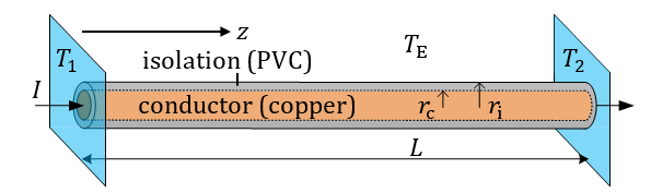
2. 1. Examined Model of a Single Cable
Figure 1 shows the modelled cable of
length ![]() ,
oriented in
,
oriented in ![]() -direction.
It consists of a solid copper conductor with radius
-direction.
It consists of a solid copper conductor with radius ![]() surrounded by an isolation (PVC).
The outer radius of the cable is
surrounded by an isolation (PVC).
The outer radius of the cable is ![]() .
An electric current
.
An electric current ![]() flows
through the cable, which is terminated with panels with infinite heat capacity
and temperature
flows
through the cable, which is terminated with panels with infinite heat capacity
and temperature ![]() respectively
respectively ![]() at the beginning respectively end.
The ambient air has the temperature
at the beginning respectively end.
The ambient air has the temperature ![]() . The coordinate
. The coordinate ![]() is
zero at the left termination.
is
zero at the left termination.
2. 2. Fundamental Thermoelectric Model for a Single Transmission Cable
The cable is modelled with a
thermoelectric equivalent circuit: Analogous to the electric domain, an
equivalent circuit of an infinitesimal short cable segment is derived as shown
in Figure 2(a). Analogous to the electric transmission line theory [13], the
differential equation is found by consideration of an infinitesimal short cable
segment. The cable parameters are all given related to length as per unit
length parameters (pul) and marked with an upstroke, e.g. ![]() .
.
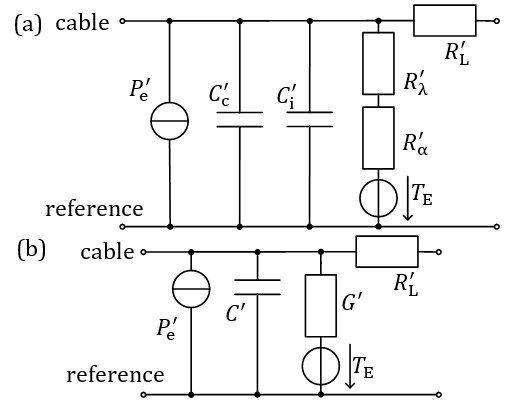
To reduce the complexity of the model, some assumptions are made in the derivation of the shown equivalent circuit: At first, the thermal conductivity of the conductor is assumed to be high, so in radial direction, the temperature gradient along the conductor is neglected and only the isolation temperature gradient remains. The isolation has a lower thermal conductivity. This is also why in axial direction, the influence of the isolation is neglected, so only the influence of the conductor remains. The following descriptions concerning the parameters are based on [9].
An overview of the calculation formulas
for the parameters is given in Table 1. The heat that is injected into the
system via the source ![]() represents the pul electrical
losses because of the electrical current
represents the pul electrical
losses because of the electrical current ![]() in
the cable. The linear temperature coefficient for the conductor conductivity is
in
the cable. The linear temperature coefficient for the conductor conductivity is
![]() .
. ![]() means the electric pul resistance
at the temperature
means the electric pul resistance
at the temperature ![]() and
and ![]() means
the conductor temperature. The thermal pul capacitances for the conductor
means
the conductor temperature. The thermal pul capacitances for the conductor ![]() and the isolation
and the isolation ![]() depend on the specific heat
capacities per volume
depend on the specific heat
capacities per volume ![]() and
and ![]() . The thermal pul resistance
. The thermal pul resistance ![]() describes the thermal heat flow
through the isolation with the thermal conductivity of the isolation
describes the thermal heat flow
through the isolation with the thermal conductivity of the isolation ![]() . The thermal pul resistance
. The thermal pul resistance ![]() is used to model the heat transfer
from the isolation to the surrounding air with convection and radiation. The
heat transfer coefficient
is used to model the heat transfer
from the isolation to the surrounding air with convection and radiation. The
heat transfer coefficient ![]() describes the radiation. The
temperatures
describes the radiation. The
temperatures ![]() and
and
![]() are the temperature of the surface
of the isolation respectively the environmental temperature in Kelvin,
are the temperature of the surface
of the isolation respectively the environmental temperature in Kelvin, ![]() is
the emissivity of the isolation material and
is
the emissivity of the isolation material and ![]() is the Stefan-Boltzmann constant.
As in [9], the emissivity is assumed to be 0.95 in this paper. The heat
transfer coefficient
is the Stefan-Boltzmann constant.
As in [9], the emissivity is assumed to be 0.95 in this paper. The heat
transfer coefficient ![]() describes free convection in air.
describes free convection in air. ![]() means the thermal conductivity of
air and
means the thermal conductivity of
air and ![]() the characteristic length of the
structure. The Nusselt number
the characteristic length of the
structure. The Nusselt number ![]() [14] is depending on the structure:
For a cylinder it is calculated using the Rayleigh number
[14] is depending on the structure:
For a cylinder it is calculated using the Rayleigh number ![]() , the Grashof number
, the Grashof number ![]() and the Prandtl number
and the Prandtl number ![]() , with the gravity of the earth
, with the gravity of the earth ![]() , the coefficient of thermal
expansion
, the coefficient of thermal
expansion ![]() and the kinematic viscosity
and the kinematic viscosity ![]() [15].
The parameters
[15].
The parameters ![]() ,
, ![]() and
and
![]() can be determined from tables as
for example given in [14] using the mean temperature
can be determined from tables as
for example given in [14] using the mean temperature ![]() , so they depend on the actual
surface temperature of the cable
, so they depend on the actual
surface temperature of the cable ![]() . In this paper,
a spline interpolation between the values given in [14] is
used. All of the aforementioned parameters describe the
radial heat flow in the cable. For the
axial behaviour, the axial thermal resistance per length
. In this paper,
a spline interpolation between the values given in [14] is
used. All of the aforementioned parameters describe the
radial heat flow in the cable. For the
axial behaviour, the axial thermal resistance per length ![]() is introduced with the thermal
conductivity of the conductor
is introduced with the thermal
conductivity of the conductor ![]() . For the calculations, the model is
condensed to the form presented in Figure 2(b). The new parameters
. For the calculations, the model is
condensed to the form presented in Figure 2(b). The new parameters ![]() and
and ![]() are calculated from the already
presented parameters.
are calculated from the already
presented parameters.
Table 1. Overview of the calculation rules for the parameters.
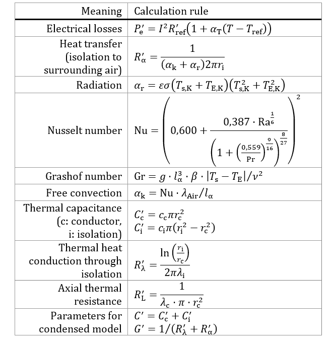
In the next step, the differential equation is deduced from the circuit model. Like in the electric domain, Kirchhoff’s laws are evaluated. Rearranging of the resulting formulas leads to the inhomogeneous partial differential equation, which describes the temperature distribution along the cable:
The elements ![]() and
and ![]() of the circuit, that lead to the
parameters of the differential equation, depend on the cable temperature. A
nonlinear differential equation results. This dependency is very complicated,
so for this moment it is neglected. Subsequently, the dependency is included by
finding a self-consistent solution using an iterative approach.
of the circuit, that lead to the
parameters of the differential equation, depend on the cable temperature. A
nonlinear differential equation results. This dependency is very complicated,
so for this moment it is neglected. Subsequently, the dependency is included by
finding a self-consistent solution using an iterative approach.
2. 3. Stationary Solution
At first, a stationary solution of
the differential equation (1) is presented. In the stationary case, there is no
variation of the temperature along the time. In the reduced differential
equation, only the variable ![]() remains.
The solution includes a homogenous and a particulate term. The constant factors
remains.
The solution includes a homogenous and a particulate term. The constant factors
![]() and
and ![]() follow from the initial conditions
follow from the initial conditions ![]() and
and ![]() (temperature at the beginning and
the end of the cable):
(temperature at the beginning and
the end of the cable):
2. 4. Complete Solution for as Single Cable
The differential equation (1) is now
solved using the Laplace transform. The temperature of the conductor at ![]() is
is ![]() . The temperature at the beginning
of the conductor is
. The temperature at the beginning
of the conductor is ![]() and at the end of the conductor
and at the end of the conductor ![]() for all times. The Laplace
transform yields
for all times. The Laplace
transform yields
The remaining differential equation
only depends on the variable ![]() and
can be solved as before. The factors
and
can be solved as before. The factors ![]() and
and ![]() are again found using the remaining
boundary conditions.
are again found using the remaining
boundary conditions.

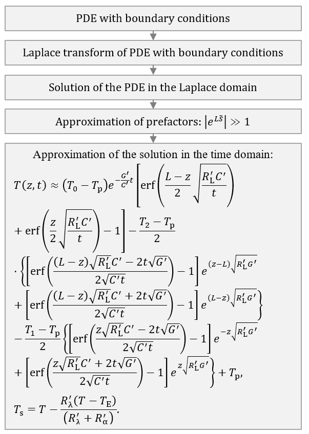
In the next step, the solution in
the Laplace domain has to be transformed back into the time domain. As numeric
inverse Laplace transformation algorithms should be avoided, an analytic
approach has to be found. There are different terms in the Laplace solution, of
which not all have a known transformation back into the time domain: The terms
in which the exponential function appears in the numerator as well as in the
denominator lead to complications. That is why ![]() and
and ![]() are approximated in the next step:
By inserting typical values, it is shown, that
are approximated in the next step:
By inserting typical values, it is shown, that ![]() can be neglected against
can be neglected against ![]() . This leads to the reduced form for
the factors:
. This leads to the reduced form for
the factors:
The approximated result in the Laplace domain can be transformed back into the time domain. The complete process of the solution including the result in the time domain is presented in Figure 3.
2. 4. 1. Infinitely Long Cable
For an infinitely long cable, only
the particulate term remains, which can be transformed back into the time
domain easily. As expected, the ![]() -dependency
vanishes:
-dependency
vanishes:
2. 4. 2. Semi-infinite Cable
In this section, a cable is
modelled, which starts at ![]() and is of infinite length. Because
of the infinite length of the cable, the factor
and is of infinite length. Because
of the infinite length of the cable, the factor ![]() has to vanish:
has to vanish: ![]() . The other factor is calculated
from the remaining boundary condition
. The other factor is calculated
from the remaining boundary condition ![]() . The inverse Laplace transform
leads to the solution in the time domain:
. The inverse Laplace transform
leads to the solution in the time domain:
3. Implementation of the Developed Solutions
In all of the before presented
solutions, constant values for the parameters in the equivalent circuit are
assumed. As one can see from the calculation rules presented in section 2. 2.,
the parameters depend on the temperatures of the conductor and the surface of
the isolation. The surface temperature of the isolation depends on the
temperature of the conductor and again of the parameters. The temperature of
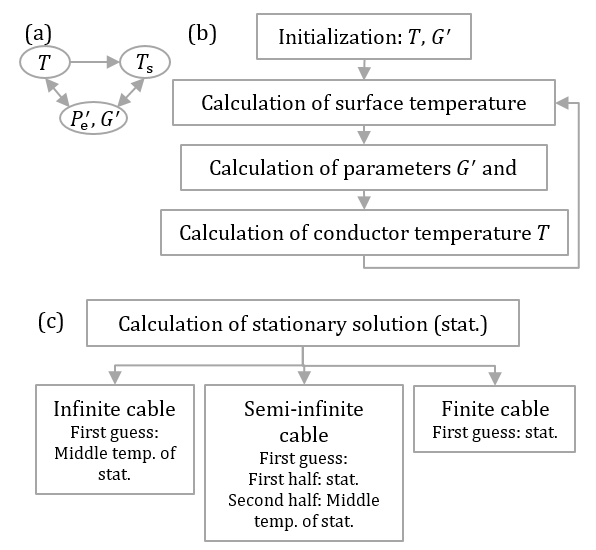
the conductor is calculated using the parameters. Those relations are shown in Figure
4(a). All in all, a self-consistent problem results. That is why an iterative
approach is used here (see Figure 4(b)): Starting with an estimated temperature
for the conductor and typical values for the parameters, the corresponding
temperature of the surface of the isolation is calculated. Using this, the
parameters are recalculated. In the last step of the first iteration, the
conductor temperature is calculated. Using this, the surface temperature is
recalculated and so on. This process is repeated a few times to find a
solution, in which parameters and the mentioned temperatures fit together.
After a few iterations (maximal 10 for the examined cases) only minor
corrections (![]() ) result from further iterations.
Generally, for each time and position along the cable, the iterations have to
be done again. This means quite some effort, if a very dense mesh of time and
space points should be calculated. But there is a huge advantage: The
temperature at each point in time and space is calculated independently from
each other point, which means, that neither the whole cable has to be
calculated if only a special point is of interest nor earlier time steps need
to be calculated if only a later point is relevant. Compared to the numeric
calculation of the solution of the differential equation this leads to an
enormous reduction of the computation time.
) result from further iterations.
Generally, for each time and position along the cable, the iterations have to
be done again. This means quite some effort, if a very dense mesh of time and
space points should be calculated. But there is a huge advantage: The
temperature at each point in time and space is calculated independently from
each other point, which means, that neither the whole cable has to be
calculated if only a special point is of interest nor earlier time steps need
to be calculated if only a later point is relevant. Compared to the numeric
calculation of the solution of the differential equation this leads to an
enormous reduction of the computation time.
In the beginning, the stationary solution is calculated. For the calculation of the infinite cable, the stationary solution in the middle of the cable is used as first guess for the temperature of the conductor. The complete solution (finite cable) as well as the semi-infinite solution depend on the time and the position along the cable. For the semi-infinite solution, the stationary temperature is used as first guess for the conductor temperature of the first half of the cable, for the second half the stationary solution in the middle of the cable is used. For the solution for the finite cable the stationary solution at the specific point of the cable is used. For each desired time the iterations are repeated until convergence is reached. As mentioned before, for the examined cases maximal 10 iterations are necessary. The complete process is summed up in Figure 4(c).
 and
the surface
and
the surface  of the cable and the parameters
  and
and  . (b) Scheme of the iterations to
include nonlinear parameters. (c) Usage of the stationary solution as first
guess for other calculations.
. (b) Scheme of the iterations to
include nonlinear parameters. (c) Usage of the stationary solution as first
guess for other calculations. 4. Numeric Reference Solution of the Partial Differential Equation
The numeric solution of the
differential equation presented in equation (1) is used to validate the
analytic approximation. The numeric solution is implemented applying the
Crank-Nicholson method and three iteration steps (see previous chapter), so
these iteration steps consider the nonlinear terms. This solution will be
regarded as correct and used as reference solution for the following
comparisons. A discretization of 100 steps for the ![]() -direction
and 1001 steps for the time is used.
-direction
and 1001 steps for the time is used.
5. Results
The presented solutions are examined
for the cable presented in Figure 1: A current of 70 A flows through a
6 mm2-cable. Therefore, the cable has the conductor radius ![]() . The total radius with isolation is
. The total radius with isolation is
![]() . The examined cable has a length of
. The examined cable has a length of
![]() . The surrounding air has the
temperature
. The surrounding air has the
temperature
![]() , which is as well the temperature
of the whole cable at
, which is as well the temperature
of the whole cable at ![]() (
(![]() ) and of the beginning (
) and of the beginning (![]() ) and the end (
) and the end (![]() ) of the cable for all times. The
conductor consists of solid copper and therefore has the specific heat capacity
) of the cable for all times. The
conductor consists of solid copper and therefore has the specific heat capacity
![]() , the thermal conductivity
, the thermal conductivity
![]() and a resistivity at
and a resistivity at ![]() of
of
![]() . The linear temperature coefficient
is
. The linear temperature coefficient
is ![]() . The isolation is made of PVC with
the specific heat capacity
. The isolation is made of PVC with
the specific heat capacity ![]() , the thermal conductivity
, the thermal conductivity ![]() and the emissivity
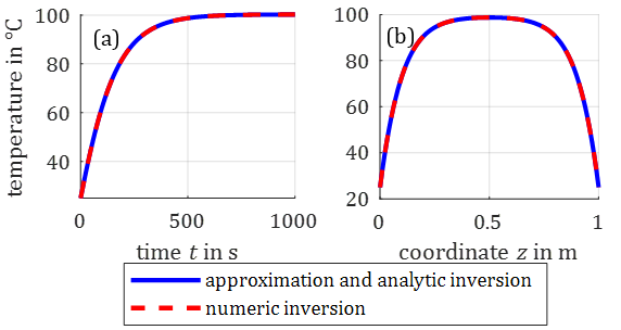
and the emissivity ![]() . The analytic approximation for the
temperature along the finite cable is compared to the numeric inversion of the
original solution in the Laplace domain to see if the approximation causes
errors. The numeric inversion of the Laplace transform is done using the
Gaver-Stehfest-algorithm [16] with the parameter
. The analytic approximation for the
temperature along the finite cable is compared to the numeric inversion of the
original solution in the Laplace domain to see if the approximation causes
errors. The numeric inversion of the Laplace transform is done using the
Gaver-Stehfest-algorithm [16] with the parameter
![]() . The results are shown in Figure 5
and differ in the fourth decimal digit. This good agreement between both
solutions confirms that the approximation is quite exact for this exemplary
setup. Therefore, the performed approximation does not cause relevant
deviations here.
. The results are shown in Figure 5
and differ in the fourth decimal digit. This good agreement between both
solutions confirms that the approximation is quite exact for this exemplary
setup. Therefore, the performed approximation does not cause relevant
deviations here.
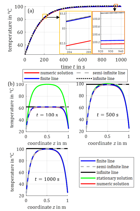
In Figure 6, the calculated results are compared to the direct numeric solution of the differential equation as presented in chapter 4. In Figure 6(a), the results for the maximum of the conductor temperature over time are shown. The temperature is taken at the middle of the cable. All analytic solutions show a similar development. For long times, the infinite and semi-infinite solutions show slightly higher values than the finite solution.
 .
. 
 , ,
, ,  .
. This is because of the length of the cable: For a longer cable, the values get closer together. The numeric solution shows a different behaviour in the transient state: Up to approximately 2 K lower temperatures are predicted here. As mentioned before, the approximation in the Laplace domain does not cause those deviations. In fact, the deviations result because in the numeric solution, the results of the iterations propagate to the next time step. As mentioned before, in the analytic solution, the calculation at each position in time and location is independent from each other position. Another function is used for each step and there is no coupling between the different positions. In the used functions, it is implicitly assumed, that all parameters are constant. That is why especially for the transient case minor deviations appear. Nevertheless, the predicted temperature only differs little from the numerically computed temperature and therefore might be used as a good, very fast approximation. In Figure 6(b), the calculated temperature along the cable is shown for different time steps. For long times, the solutions get closer together and meet the stationary solution. In the transient area, the numeric and analytic approaches slightly deviate from each other mainly in the middle of the cable.
6. Conclusion
In this contribution, a new analytic
approach for the transient axial temperature distribution along a single cable
with constant ambient temperature and fixed temperatures at the beginning and
the end of the cable is presented. The cable is assumed to have a constant
temperature at the beginning ![]() . Using an iterative approach,
non-linear material parameters can be considered. Compared to known numeric
solutions for this configuration, a significant reduction of the calculation
time is achieved. The solution is very close to the numeric solution, so it can
be used for example in smart fuses. Furthermore, solutions for cables of
infinite length are presented. The usage of the semi-infinite cable reduces the
effort of the computation even further and might be used when accuracy can be
lower and computational resources are reduced.
. Using an iterative approach,
non-linear material parameters can be considered. Compared to known numeric
solutions for this configuration, a significant reduction of the calculation
time is achieved. The solution is very close to the numeric solution, so it can
be used for example in smart fuses. Furthermore, solutions for cables of
infinite length are presented. The usage of the semi-infinite cable reduces the
effort of the computation even further and might be used when accuracy can be
lower and computational resources are reduced.
References
[1] S. Önal and S. Frei, “A model-based automotive smart fuse approach considering environmental conditions and insulation aging for higher current load limits and short-term overload operations,” in IEEE International Conference on Electrical Systems for Aircraft, Railway, Ship Propulsion and Road Vehicles & International Transportation Electrification Conference (ESARS-ITEC), Nottingham, United Kingdom, 2018. View Article
[2] R. Olsen, G. J. Anders, J. Holboell and U. S. Gudmundsdóttir, “Modelling of Dynamic Transmission Cable Temperature Considering Soil-Specific Heat, Thermal Resistivity, and Precipitation,” in IEEE Transactions on Power Delivery, 2013, vol. 28, no. 3, pp. 1909–1917. View Article
[3] C. Holyk, H.-D. Liess, S. Grondel, H. Kanbach and F. Loos, “Simulation and measurement of the steady-state temperature in multi-core cables,” in Electric Power Systems Research, 2014, vol. 116, pp. 54–66. View Article
[4] M. Lei, G. Liu, Y. Lai, J. Li, W. Li and Y. Liu, “Study on thermal model of dynamic temperature calculation of single-core cable based on Laplace calculation method,” in IEEE International Symposium on Electrical Insulation, San Diego, CA, 2010. View Article
[5] D. Lauria, M. Pagano and C. Petrarca, “Transient Thermal Modelling of HV XLPE Power Cables: matrix approach and experimental validation,” in IEEE Power & Energy Society General Meeting (PESGM), Portland, OR, 2018. View Article
[6] Q. Zhan, J. Ruan, K. Tang, L. Tang, Y. Liu, H. Li and X. Ou, “Real-time calculation of three core cable conductor temperature based on thermal circuit model with thermal resistance correction,” in The Journal of Engineering, 2019, vol. 2019, no. 16, pp. 2036–2041. View Article
[7] L. Brabetz, M. Ayeb and H. Neumeier, “A New Approach to the Thermal Analysis of Electrical Distribution Systems,” in SAE 2011 World Congress & Exhibition, Detroit, MI, 2011. View Article
[8] R. S. Olsen, J. Holboll and U. S. Gudmundsdóttir, “Dynamic Temperature Estimation and Real Time Emergency Rating of Transmission Cables,” in IEEE Power and Energy Society General Meeting, San Diego, CA, USA, 2012. View Article
[9] S. Önal, M. Kiffmeier and S. Frei, "Modellbasierte intelligente Sicherungen mit umgebungsadaptiver Anpassung der Auslöseparameter," in International Conference EEHE, Electric & Electronic in Hybrid and Electric Vehicles and Electrical Energy Management, Würzburg, Germany, 2018.
[10] F. Loos, K. Dvorsky and H.-D. Liess, “Two approaches for heat transfer simulation of current carrying multicables,” in Mathematics and Computers in Simulation, 2014, vol. 101, pp. 13-30. View Article
[11] J. He, Y. Tang, B. Wei, J. Li, L. Ren, J. Shi, K. Wu, X. Li, Y. Xu and S. Wang, “Thermal Analysis of HTS Power Cable Using 3-D FEM Model,” in IEEE Transactions on applied superconductivity, 2013, vol. 23, no.3. View Article
[12] S. L. Rickman and C. J. Iannello, “Heat transfer analysis in wire bundles for aerospace vehicles,” in International Conference on Simulation and Experiments in Heat Transfer and its Applications, Ancona, Italy, 2016. View Article
[13] C. R. Paul, Analysis of multiconductor transmission lines. 2. ed., Piscataway, NJ: IEEE Press, 2008.
[14] VDI-Gesellschaft Verfahrenstechnik und Chemieingenieurwesen, VDI-Wärmeatlas. Berlin: Springer, 2013.
[15] S. W. Churchill and H. H. Chu, “Correlating equations for laminar and turbulent free convection from a horizontal cylinder,” in International Journal of Heat and Mass Transfer, 1975, vol. 18, no. 9, p. 1049–1053. View Article
[16] J. Abate and W. Whitt, “A Unified Framework for Numerically Inverting Laplace Transforms,” in INFORMS Journal on Computing, 2006, vol. 18, no. 4. View Article