Journal of Fluid Flow, Heat and Mass Transfer (JFFHMT)

ISSN: 2368-6111

Nomenclature

1. Introduction

The distribution and preparation of sanitary hot water in Belgrade takes place 24 hours a day, but with very different levels of intensity during the 24 hours. The highest consumption of this water in apartments is during the early morning and evening hours, as shown in the diagram [1].

The diagram shows that in these intervals the consumption of this water increases many times over. With the view of determining the actual hydraulic modes in the domestic hot water (DHW) preparation system [2], continuous measurement of fluid temperatures in the primary and secondary DHW installations was carried out under realistic operating conditions [3],[4], with all volumes of consumption of this water and lengths of their duration.

Measurements of the fluid flow also show that the existing control equipment must react in several ways over a period of 1 second, causing hydraulic impacts in the heat substations and the complete heating system.

Also, from the diagram, it can be seen that during the night hours, there is practically no consumption of sanitary hot water.

The significant inconsistency of the flow of fluids detected in the course of the delivery of sanitary hot water has caused many problems, such as insufficient delivery of sanitary hot water in "peak" loads, hydraulic strikes and vibrations in the heat substations, and contamination of the plate heat exchangers used for heating this water as a result of the hibernation of the fluid in the night mode.

Therefore, the flow model in the mentioned heat exchangers was developed in order to find solutions for the identified problems.

Regarding the determination of boundary conditions, in addition to the standard boundary conditions stated in this paper, it was necessary to adopt a turbulence flow regime in the channels, and within it a standard k-ε turbulence model.

As mentioned earlier, other models of turbulence could not be applied because they were not able to achieve the results of testing turbulence parameters for the adopted flows.

It should be noted that other turbulences models did not accept the stated fluid flow values as the initial boundary conditions and therefore could not be applied in this case.

1.1 k-ε Model

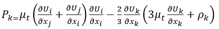
k is the turbulence kinetic energy and is defined as the variance of the fluctuations in velocity. It has dimensions of (m ²/sec ²); for example, m² /s²  is the turbulence eddy dissipation (the rate at which the velocity fluctuations dissipate), and has dimensions of per unit time(m ²/sec ³)[5].

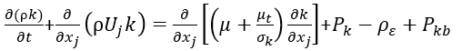
The k–ε model introduces two new variables into the system of equations

The values of k and ε come directly from the differential transport equations for the turbulence kinetic energy and turbulence dissipation rate.

1.2. Reynolds Number

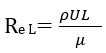
where,

1.3. The Basic Boundary Conditions

The basic boundary conditions for exchange of heat and flow of fluid are as follows[5]
-FLUID 1- input, FLUID 2- input :
The mass influx is calculated using:

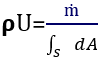
Where
-is the integrated boundary surface area at a given mesh resolution;
–U, m/sec, velocity magnitude;
–, kg/m³, density.
-FLUID 2- input:
-Mean value of static pressure.

The Reference Pressure (Eqn. 7) is the absolute pressure data from which all other pressure values are taken.

ANSYS CFX [5]solves for the relative static pressure-(thermodynamic pressure)(Eqn.8) in the flow field, and is related to Absolute Pressure-(Eqn.9):

-The input temperature

The total Temperature, the boundary advection and diffusion terms for specified total temperature, are evaluated in exactly the same way as specified static temperature, except that the static temperature is dynamically computed from the definition of total temperature:

For a fluid with a constant heat capacity this value is:

2. Problem Statement

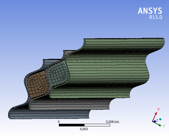
Modelling was done for individual channels between the profiled plate, whose cross section is shown in the following figures:

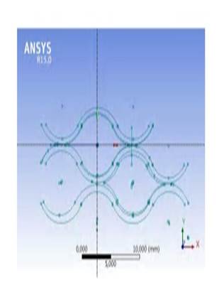
The equivalent cross-sectional diameter of the channel is 4.88mm, and the lengths of shorter and longer diagonals are 4 mm and  8.2 mm[3].

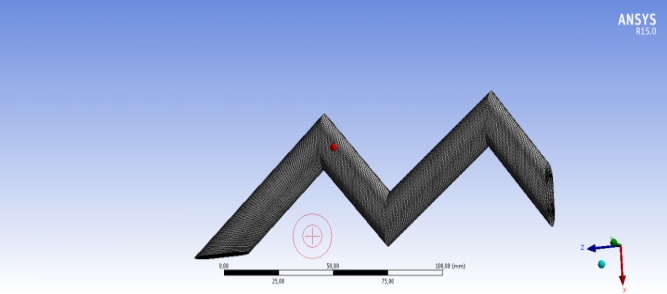
The individual plate channels are drawn in threedimensional software Design Modeler and may be shown as rectilinear channels (Figure 2.) and chevron type channels (Figure 3.).

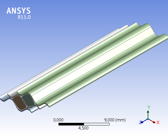
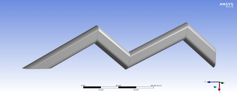
In these individual plate channels, fluid velocity on both sides of the plate was identical and amounted to 0.01 m / sec or 0.1 m/sec.

2.1. Numerical network

For all channel surfaces through which fluid flow occurs and heat exchange is conducted, numerical networks are generated and their input-output crosssections for the fluid flow are numbered using the standard softwares module.

The characteristics of the numerical networks depended on the adopted velocities at inlet channel intersections. These networks were generated for the adopted volumetric flow rate, ranging from 0.01 m/s to 0.1 m/s. Outside this velocity range, it not possible to generate these networks due to the occurrence of the velocities of the reverse flow of the fluid.

The characteristics of these networks (number of nodes, density) have directly preconditioned the feasibility of the results obtained related to fluid flow process parameters (with)in the post-process investigations framework.

Thus, for example, in the turbulent mode (exchange of the kinetic energy, Reynolds Number values) it was not possible to obtain the results for the modeled process parameters for the assumed velocity of 0.01 m/s. Thus, for the purpose of this paper, iterative procedures within the initial boundary conditions were assumed to be ten times the velocity of the fluid.

A numerical network is generated for this panel, as shown in the following figure:

2.2. The basic boundary conditions

The basic boundary conditions for exchange of heat and flow of fluid are as follows:
-FLUID 1- input, FLUID 2-input:
The mass of fluid flow or fluid flow rate between the plates of the exchangers during the heat exchange for both fluids have adopted values of 0.1 m/sec, 0.05m/sec and 0.01m/sec .
- FLUID 2- input:
The mean value of static pressure of 550, 000Pa.
- The input temperature of the fluid during periods of heat exchange of 65 ° C for Fluid 1 and 50 ° C for heated Fluid 2.

2.3. Modeling results

2.3.1.Modeling results of turbulence phenomena in rectilinear channels

All modeling results have been realized in the ANSYS software (CFD and CFX modules) [5] and are presented in diagrams with parameter values that cannot be changed because they refer only to one predetermined number of iterations of the parameter of the process of fluid flow and heat exchange.

Also, within the obtained diagrams, there can be no change in the number or character of curves indicating the indicated iterations.

For the assumed laminar flow within the boundary conditions of the CFX module, results of the channel flow intensity diagrams within the boundary layer were obtained.

Contours of Velocity Magnitude as shown in the following Figures 6. and Figures 7.

From these figures, it can be observed that the maximum fluid velocities in the laminar mode are in the contour center surfaces of the channel, and these velocities are gradually decreasing towards the zones where the two plates of the exchanger are connected. This is particularly related to flow speed of 0.1m/s where the contour velocities in the central (widest) section of the channel intersection are ten or twenty times larger compared to the contour surfaces of the flow current at the junction of the two plate exchangers forming the channel.

For the assumed turbulent flow mode under the initial boundary conditions of the CFX-module, intensity diagrams of the channel flow have not been met, i.e., Contours of Velocity Magnitude at turbulent flow of fluid at a velocity of 0.01m/s and at a velocity of 0.1m/s have a zero value.

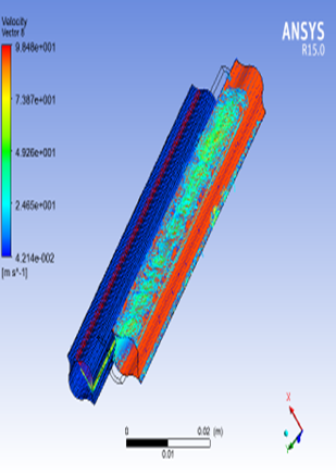
Within the post-process research [5], the values of the collecting velocities of fluid flow in the contour surface of the channel as well as the flow velocities in the intersection of the channel were determined, as shown in the following Figure 8. and Figure 9.

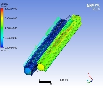
Both diagrams are the result of the assumed laminar flow.

The contour surfaces of dark blue (Figure 8.), in which the flow velocity is zero, represent "dead zones" - at the point of contact of two panels of the channel. It should be noted that these “dead zones“ occur at inlet flow velocities of 0.01m/s within the intersection zone of two channel-forming exchanger plates.

Within the post-process research of fluid velocity (within the boundary surfaces of fluid current flow)for assumed turbulent flow in the channels at the same input velocities of 0.01m/sec and 0.1m/sec, the velocities of several hundred thousand m/sec were obtained along these rectilinear channels. However, as such velocities may not be achieved, these results have not been published.

The contours of cell Reynolds Number is also shown in the following Figure 10.

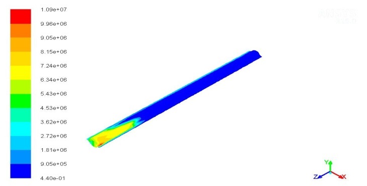
The contours of cell Reynolds Number at laminar flow of fluid at a velocity of  0.1m / sec (0.4–10000000) have almost the same value as at the velocity of 0.01m/sec.

It was not possible to obtain the results of changes with low Reynolds Number values in kinetic flow energies along channels for laminar fluid flow performed during post-process investigations and CFX module.

2.3.2. Modeling  Results of Turbulence Phenomena In Chevron Type Channels

In the CFX module , it was not possible to show the values of the realized kinetic energy of the fluid and Cell Reynolds Numbers in the chevron type channels.

Although the fluid flow charts were obtained for this type of channel, results are insufficient in terms of velocity changes at points of abrupt change of fluid flow direction (Figure 8).

Therefore testing was performed of the applied kinetic energy changes of fluid flow in the contour layer along the entire path through the tester (chevron) channels and their inlet-outlet sections.

These values are shown in the diagrams of the  Fluent module in all positions of the fluid flow in this type of channel.

Position(m) on the abscissa of the diagram represents the distance of any point of the channel from the input section.

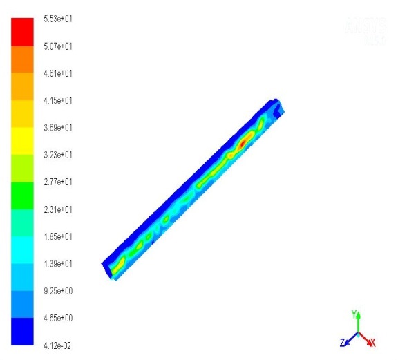
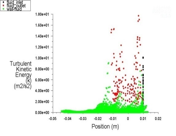
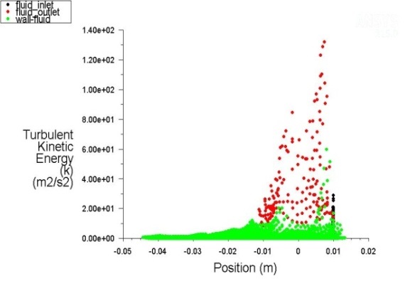
The following figures (Figure 11., Figure 12., Figure 13., Figure 14.,   Figure 15. and Figure 16.) show changes in the intensity of the kinetic energy and Reynolds Number for the different regimes of fluid flow along the channel.

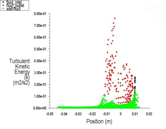
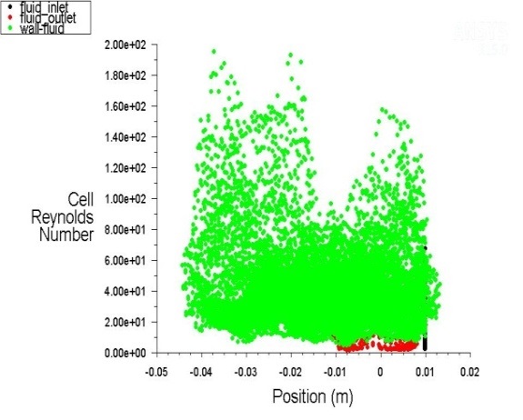
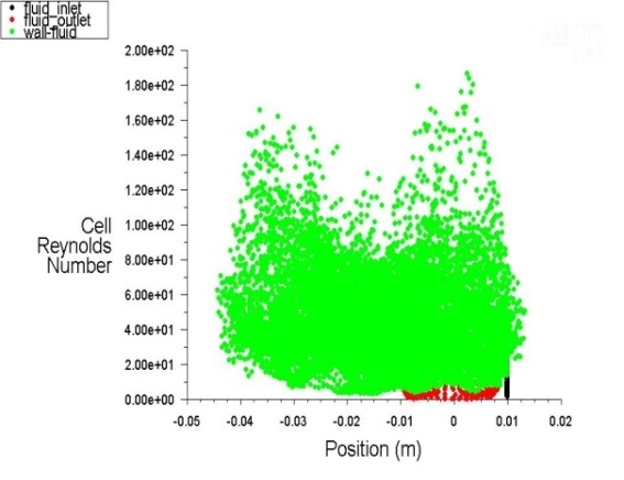
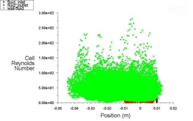
The lowest values of the Reynolds number are in the straight-line section of the channels for all three hydraulic modes, where there are also the lowest velocities of fluid flow. These values increase towards the fluid inlet and outlet cross-sections.

It is also noted that the values of the exchanged kinetic energy of the surface boundary layers of the fluid flow are lower along the perpendicular path sections than at points of abrupt flow direction changes and applicable to all three flow modes.

At the same time extreme upsurge of exchanged kinetic energy of the boundary surface layers of the fluid flow are recorded at points of abrupt flow direction changes and applicable to all three flow modes.

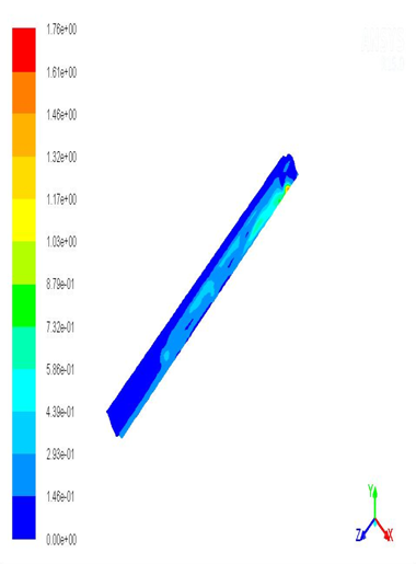
The following figure shows the change in the velocity profile of the fluid flow along the chevron type channel.

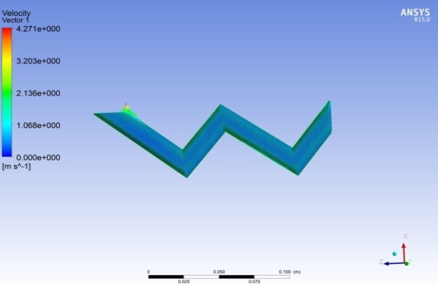
The diagram shows the change of intensity of the flow velocity from the central part of the cross-section of the fluid flow related to the boundary surface flow and a certain increase of the flow velocities at the constriction point of the fluid flow section.

3. Results and Discussions

The modeling results of turbulence phenomena have been achieved for the previously assumed laminar flow regime of fluids in rectilinear channels and for the previously assumed turbulent regime of fluid flow of in shevron type channels.

3.1. Results and Discussions –Rectilinear Channels

The results obtained in the rectilinear channels have shown local turbulent phenomena such as the reverse flow of fluids in the transient convex-concave region of the channel cross-section (Figure 1.) when changes in fluid velocity fluctuations can be described most closely by the sinusoidal curve[3].

In addition, in the zone of connection of the two plates of the exchangers that form the channel, there is a standstill of the fluid, where the velocity is zero and where there are conditions for contamination of the plates.

Despite these local turbulent phenomena, Reynolds numbers of fluid flows along the rectilinear channel have an extremely low value - around zero, except in a very small part of the channel intersection, when this value is only locally multiplied (Figure 10.).Therefore, it can be argued with reliability that fluid flow in rectilinear channels is laminar.

3.2. Results and Discussions –Chevron Type Channels

The modeling results of the kinetic energy of the fluid flow show for the assumed values of the fluid velocity (from 0.01 m/sec to 0.1 m/sec) extremely low values - from 80 m²/sec²  to 140 m²/sec². The values of Reynolds numbers are in the range of 200 to 300 (Figure 12., Figure 14. and Figure 16.).Therefore, it can be argued with reliability that the flow in the chevron type channels is laminar, although in the initial boundary conditions the turbulent flow regime was assumed to correspond to the k-ε turbulence model.

It can also be said that at the above assumed fluid velocities, there are no large changes in the intensities of fluid velocities in the chevron type channels, and it may be assumed that they gradually increase from the center of the intersection of these channels towards the contour surfaces(Figure 17).
This is in contrast to the study of these channels conducted by Dafe Eregregor [6], where, in the hydraulic modes with Reynolds intervals ranging from 2300 to 10000, the changes in fluid velocities in the rounded sections of the chevron type channels are more prominent so that the flow becomes turbulent in nature.

On the basis of everything stated, it has been found that the flow regime of fluids in the heat exchanger channels for the preparation of sanitary hot water is laminar, and that the individual zones of hydraulic flow unsteadiness cannot be classified under any of the standard turbulence models.

By examining the large zonal hydraulic unsteadiness caused by the jump in the flow of sanitary domestic hot water and, consequently, the fluid which heats it, and by observing the hibernation of the fluid during the night, it can be concluded that all the preconditions are met for contamination and a decrease in the thermal function of these devices[1], as well as for their thermal inefficiency at "peak" consumption of sanitary hot water when they cannot meet the needs of consumers.

3.3. Validation Of Results

Confirmation of modeling results is their comparison with the results of measuring fluid flow parameters and heat exchange in different parts of thermal substations obtained in all regimes of domestic hot water heating [1], [7]. Therefore, the above laws achieved by modeling are confirmed.

This is especially true for "dead zones" in individual channels in which very small values of flow velocities, which are very close to zero, are obtained by numerical simulations. At the same time, in the collective channels of the exchanger from which the individual channels are supplied, very low speeds (from 0. 005 m / sec to 0.01 m / sec) were confirmed by measurements [3].

It should be noted that from these aggregate channels, the total fluid flow is distributed to 96 individual channels (for the plate heat exchanger test model), so it is logical to expect that the flow in individual channels is approximately 96 times lower, and practically zero, which is confirmed by the numerical method.

At the same time, at peak loads in domestic hot water consumption in the morning and evening, with frequent occurrence of hydraulic shocks [1], fluid  flows could not be measured in the collection channels. At the assumed velocities in the aggregate channels higher than 0.1 m / sec and for the assumed turbulent flow regime, it was not possible to obtain the results of fluid flow velocities in individual channels by numerical simulations, which is stated in the section "2.3.1.Modeling results of turbulence phenomena in rectilinear channels ".

4. Conclusion

All results of numerical simulations of fluid flow velocity in variable (peak) regimes are absolutely consistent with the results of measurements of this velocity in thermal substations at different levels of hydrostatic fluid pressures represented in variable modes[4], [7].

The established laminar flow of fluids in the channels and the existence of dead zones imposes a need for the introduction of new project procedures for the selection of these channels, considering the assumed accumulated values of the speeds in the inlet channel crossings (0.01m/sec and 0.1m/sec).

Moreover, it can be said that the established laminar flow regime in the channels refers to the nominal regimes of the domestic hot water consumption, which are at their longest during the day, indicating insufficiently efficient heat exchange through the plate heat exchanger.

However, due to the very low flow velocities in the real sections of the ducts and consequently the low values of the tangential voltages, there is still a risk that the heat exchanger plates may become soiled, and, consequently, the thermal function of these appliances may fall.

According to [3] it is not recommended to size the heat exchanger with the shear stress below 50 Pa, and if there is a significant risk of fouling it is recommended that the shear stress should be increased to at least 100 Pa.

The design procedure for the selection of the passage of the fluid should take into account the fact that the surface of the channels in the area of the "dead zone" is seeping off - at the point of connection of the two boards of the exchanger, resulting in a drop in the heat function of the exchanger [7].

CFD modeling of turbulent phenomena in plate heat exchanger channels indicates the necessity of its application in maintaining the thermal function of these devices during the period of exploitation. Such an analysis imposes the need to introduce periodic interruption of the operation of the exchangers for the heating of domestic hot water and the need for parallel introduction of additional heat exchangers for "peak" loads.

The need for additional analyses of the justification for the implementation of individual night switch-offs and the inclusion of additional heat exchangers during the "peak" loads arises from the huge costs of exploiting and maintaining these combined systems for heating sanitary hot water and the ever-increasing demands for improving the quality of its delivery.

The results of the numerical simulations have provided a very realistic picture of fluid flow to such an extent that they impose themselves as an indispensable method in the study of the aforementioned hydraulic phenomena.

Several hydraulic phenomena have not been sufficiently addressed in this paper since they were discovered during the research of standard hydraulic phenomena applicable to fluid flow through duct walls.  

A major advantage of this method is its application to variable operating conditions, which is achieved by changing the initial boundary conditions of the calculation, thus creating the conditions for a comprehensive overview of the process.

This is one of the main reasons why all non-stationary phenomena can be localized and classified into standard mathematical models.

References

[1] Goteborg Energy, Public Utility Company “Belgrade Power Plants”, District Heating System Rehabilitation Program in Belgrade, Belgrade, Serbia, June 2004.
[2] Public Utility Company “Belgrade Power Plants”, Rules on the Operation of the Heat Distribution System, Official Journal of the City of Belgrade No.54 / 2014, Belgrade, Serbia, 2014.
[3] Srbislav B. Genić, Branislav M. Jaćimović, Dragan N. Mandić, Dragan Petrović, Experimental determination of fouling factor on plate heat exchangers in district heating system, Energy and Buildings 50(2012) 204-211.View Article
[4] Dragan Mandic, CFD modeling of turbulence in channels of plate heat exchangers, 5th International Conference of Fluid Flow, Heat and Mass Transfer.
[5] ANSYS Introduction to CFD Analysis, Notes, FLUENT v 6.3, December 2006.
[6] Dafe Eregregor, Numerical simulation of Heat Transfer and Pressure drop in channels of Plate Heat Exchangers using Fluent as a CFD tool, Department of mechanical engineering, Blekinge Institute of Technology, Karlskrona, Sweden, 2008.
[7] Dragan Mandic, Study of the Impact of Work Fluid Contamination on Heat Exchange Intensity in Plate Heat Exchangers in District Heating, Doctoral Thesis, Belgrade, Serbia, 2011.