Journal of Fluid Flow, Heat and Mass Transfer (JFFHMT)
ISSN: 2368-6111

Volume 7 - Year 2020 - Pages 1-11
DOI: 10.11159/jffhmt.2020.001
Solid-Liquid Phase Change in the Presence of Gas Phase: Numerical Modeling and Validation
Ravi Govindram Kewalramani, Sebastian Pose, Ingo Riehl, Tobias Fieback
Institute of Heat Engineering and Thermodynamics, Chair of Technical Thermodynamics,
TU Bergakademie Freiberg
Gustav-Zeuner-Str. 7, 09599 Freiberg/Sachsen, Germany
Ravi.Kewalramani@ttd.tu-freiberg.de; Sebastian.Pose@ttd.tu-freiberg.de;
Ingo.Riehl@ttd.tu-freiberg.de; Tobias.Fieback@ttd.tu-freiberg.de
Abstract - In the present work a fundamental numerical model is implemented in the open source framework, finite volume method (FVM) based computational fluid dynamics (CFD) program OpenFOAM®, to tackle the solid-liquid phase change phenomena in the presence of gas phase. The volume of fluid (VoF) method is employed to distinguish between the phase change material (PCM) and the gas phase, and the enthalpyporosity method is adopted to capture the moving boundary phase change phenomena in the PCM. The discussed model is validated against the well documented cases in the literature i.e., 1D Stefan problem, melting of gallium and free surface thermocapillary flow with phase change. The simulation results are in very good agreement with those found in the literature. Finally, experiments are performed with partially filled paraffin wax (Rubitherm® RT31) in the presence of air in an enclosure. The left and right walls of the enclosure are made of aluminum plates and maintained at different temperatures while the remaining walls are made of Plexiglas. The temporal evolution of the melting front during melting obtained from the discussed numerical model is compared with experiments.
Keywords: CFD, Enthalpy-porosity method, Multiphase flows, OpenFOAM®, PCM, Solid-liquid phase change, Thermocapillary flow, VoF.
© Copyright 2020 Authors - This is an Open Access article published under the Creative Commons Attribution License terms Creative Commons Attribution License terms. Unrestricted use, distribution, and reproduction in any medium are permitted, provided the original work is properly cited.
Date Received: 2019-10-31
Date Accepted: 2020-01-31
Date Published: 2020-03-05
Nomenclature:
| Latin Symbols | ||
| Mushy zone constant | kg m−3 s−1 | |
| Specific heat capacity | J kg–1 K–1 | |
| Gravity vector | m s−2 | |
| Specific enthalpy | J kg–1 | |
| Latent heat | kJ kg–1 | |
| Pressure | Pa | |
| Buoyancy source term | kg m−2 s−2 | |
| Darcy type source term | kg m−2 s−2 | |
| Surface tension force term | kg m−2 s−2 | |
| Surface area | m | |
| Time | s | |
| Temperature | K | |
| Velocity vector | m s–1 | |
| Greek Symbols | ||
| Volume fraction | - | |
| Thermal diffusivity | m2 s−2 | |
| Coeff. Of thermal expansion | K–1 | |
| Melt fraction | - | |
| Thermal conductivity | W m–1 K–1 | |
| Eigenvalue | - | |
| Density | kg m–3 | |
| Dynamic viscosity | kg m–1 s–1 | |
| Subscripts | ||
| c | Cold | |
| Ref | Reference | |
| liq | Liquidus | |
| sol | Solidus | |
| m | Melt | |
| h | Hot | |
| Abbreviations | ||
| CFD | Computational Fluid Dynamics | |
| DSLR | Digital Single Lens Reflex | |
| LED | Light Emitting Diode | |
| PCM | Phase Change Material | |
| RT | Rubitherm® | |
| VoF | Volume of Fluid | |
1. Introduction
The solid-liquid phase change in the presence of third phase (liquid or gas) is of the utmost importance in many industrial processes such as casting, welding, thermal storage systems, powder atomization, etc. Therefore, the understanding of solidification and melting, its initial and thermal conditions plays a crucial role to make the process more efficient. Over the past few decades numerical simulations of solid-liquid phase change is gaining popularity in the industry not only to improve the quality of their products, but also to make cost effective manufacturing decisions [1]. A common approach for modeling such multi physical phenomena is coupling of Volume of Fluid (VoF) method with a solid-liquid phase change model in Eulerian frame.
Since the introduction of the enthalpy method by Voller et al. [2], several numerical methods, formulations and models have been found in the literature to tackle the solid-liquid phase change phenomena and especially in handling of the velocity field in the solid phase. Hu and Argyropoulos [3] reviewed various methods and stated the pros and cons of the discussed methods according to the nature of the problem and computational expenses. Rösler and Brüggemann [4] developed a numerical model to study the melting process of phase change material (PCM) in latent heat storage systems and incorporated an error function to describe the melt fraction. Miehe [5] implemented and compared the viscosity and Darcy model to investigate the twin-roll casting process of the magnesium alloy. Kasibhatla et al. [6] adopted the variable viscosity model to study the melting and settling of PCM in a capsule. More recently König-Haagen et al. [7] performed a comprehensive benchmarking of fixed-grid methods and presented a qualitative and quantitative analysis of most common energy formulations for the modeling of melting.
The VoF approach proposed by Hirt and
Nichols [8] is
the well-known interface-capturing technique, which uses an indicator function
to mark different fluids. This approach has also been previously used for the
solid-liquid phase change simulations in a multiphase system. Assis et al. [9]
performed parametric CFD analysis of melting process of PCM (Rubitherm® RT27)
in a partially filled spherical shell. The VoF method was employed to account
for PCM-air system and the enthalpy-porosity method was adopted for the solid
liquid phase change. A temperature dependent density function![]() was used for air phase, whereas a
variable density based on Boussinesq approximation was implemented in the
liquid PCM.
was used for air phase, whereas a
variable density based on Boussinesq approximation was implemented in the
liquid PCM.
Shmueli et al. [10] investigated the influence of the large mushy zone constant ![]() in
vertical cylindrical tube, partially filled with PCM (RT27) with a flat
surface. A temperature dependent viscosity function
in
vertical cylindrical tube, partially filled with PCM (RT27) with a flat
surface. A temperature dependent viscosity function ![]() and variable density
and variable density ![]() were
used in the liquid PCM. Two sets of thermophysical properties were examined, at
first uniform values of specific heat capacity (
were
used in the liquid PCM. Two sets of thermophysical properties were examined, at
first uniform values of specific heat capacity (![]() and thermal conductivity
and thermal conductivity![]() for solid and liquid phase was
assigned, later a small variation of thermal conductivity between phases was
considered (i.e.
for solid and liquid phase was
assigned, later a small variation of thermal conductivity between phases was
considered (i.e.![]() ). Rösler [11]
investigated close contact melting of a PCM with air above it in a capsule. The
PCM was assumed to be an incompressible fluid, whereas the gas phase (air) was
modeled as a compressible fluid. Similarly, Kasibhatla et al. [12]
also investigated the close contact melting in a capsule using a multiphase
approach and variable viscosity model to enforce the velocity in the solid
region to zero.
). Rösler [11]
investigated close contact melting of a PCM with air above it in a capsule. The
PCM was assumed to be an incompressible fluid, whereas the gas phase (air) was
modeled as a compressible fluid. Similarly, Kasibhatla et al. [12]
also investigated the close contact melting in a capsule using a multiphase
approach and variable viscosity model to enforce the velocity in the solid
region to zero.
Furthermore, Tan et al. [13] performed simulations in small scale geometries to investigate the effects of thermocapillary convection and the dynamics of the gas phase during the solidification of pure bismuth with an argon gas on the top using a multiphase approach. Saldi [14] studied the Marangoni driven free surface hydrodynamics in liquid steel weld pools during solid-liquid phase change with free surface deformation. Finally, Richter et al. [15] performed mold filling and solidification simulations; the gas phase was treated as an incompressible fluid with constant properties. A special treatment was employed to handle the Darcy-type source term at the interface between PCM and air.
As evident from the above literature research, the coupling of VoF Method with the enthalpy porosity method is an effective way to tackle such multi-physical phenomena numerically. Therefore, in this study a fundamental numerical model of solid-liquid phase change in the presence of gas phase is presented. The PCM and gas phase are considered as two-phase immiscible incompressible fluid and are modeled using the VoF [8] approach based on interface capturing method. A fixed grid enthalpy-porosity method [16, 17] is employed for the solid-liquid phase change. Thermophysical properties of both the fluids are constant and independent of temperature. The Boussinesq approximation is used for both the fluids (liquid PCM and air).
2. Numerical Model
2. 1. Governing Equations
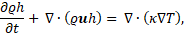
The solid-liquid phase change with a free surface is handled by solving the governing equations discussed in this section, using a single domain formulation. The conservation equations accounts for both the differences in fluid properties as well as surface tension forces acting at the interface. The mass, momentum and energy conservation equations are given by [13, 14, 16, 17]:


where ![]() is the velocity vector, t the time, p
the pressure,
is the velocity vector, t the time, p
the pressure, ![]() the
density,
the
density, ![]() the
dynamic viscosity,
the
dynamic viscosity, ![]() the
specific enthalpy, T the temperature,
the
specific enthalpy, T the temperature, ![]() the
thermal conductivity,
the
thermal conductivity, ![]() the buoyancy source term,
the buoyancy source term, ![]() the surface tension force term,
the surface tension force term, ![]() the Darcy type source term.
the Darcy type source term.
2. 2. Volume of Fluid (VoF) method
The VoF uses an indicator function ![]() to mark different fluids:
to mark different fluids:
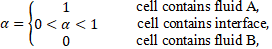
in the present work fluid A is the PCM and fluid B is the gas phase. The volume fraction α transport equation can be written as:
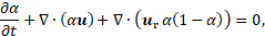
where![]() , is the relative velocity between two
fluids. On the contrary to the classical VoF method originally proposed by Hirt
and Nichols [8],
the VoF method in OpenFOAM® uses an additional convective term also referred to
as the artificial compression term (the third term in Eq.(5))
to minimize the numerical diffusion at the interface [18].
This term is only active within the cells containing interface due to its
dependence on
, is the relative velocity between two
fluids. On the contrary to the classical VoF method originally proposed by Hirt
and Nichols [8],
the VoF method in OpenFOAM® uses an additional convective term also referred to
as the artificial compression term (the third term in Eq.(5))
to minimize the numerical diffusion at the interface [18].
This term is only active within the cells containing interface due to its
dependence on ![]() where
where ![]() (0, 1). The relative velocity also
known as the compression velocity
(0, 1). The relative velocity also
known as the compression velocity![]() is computed by:
is computed by:
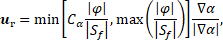
where ![]() is the fluid flux,
is the fluid flux, ![]() surface area and
surface area and ![]() compression coefficient. In the
present work
compression coefficient. In the
present work ![]() is set to 1. The thermophysical
properties of each fluid are expressed in terms of volume fraction
is set to 1. The thermophysical
properties of each fluid are expressed in terms of volume fraction![]() :
:
where ![]() is either
is either![]() .
.
The surface tension force term ![]() in Eq. (2) is
the continuum surface force (CSF) model proposed by Brackbill et al. [19]
and is expressed as:
in Eq. (2) is
the continuum surface force (CSF) model proposed by Brackbill et al. [19]
and is expressed as:

where ![]() is
the surface tension and
is
the surface tension and ![]() the surface curvature. The surface
curvature is defined as:
the surface curvature. The surface
curvature is defined as:

2. 3. Solid-liquid phase change
The specific enthalpy ![]() in
Eq. (3)
can be defined as the sum of sensible heat and latent heat, such that:
in
Eq. (3)
can be defined as the sum of sensible heat and latent heat, such that:
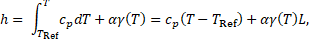
where ![]() is the specific heat,
is the specific heat, ![]() the reference temperature,
the reference temperature, ![]() restricts
the term in fluid A (PCM),
restricts
the term in fluid A (PCM), ![]() the melt fraction as a function of
temperature and
the melt fraction as a function of
temperature and ![]() the latent heat of fusion.
the latent heat of fusion.
By combining Eq. (3) and Eq. (10), we get the energy conservation equation in terms of temperature, as shown below:

The melt
fraction ![]() [0, 1] is defined as a linear
function of temperature:
[0, 1] is defined as a linear
function of temperature:
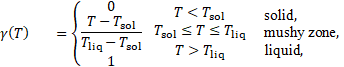
where ![]() is the solidus temperature and
is the solidus temperature and ![]() the liquidus temperature.
the liquidus temperature.
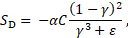
The Darcy
type source term ![]() in Eq. (2) is
modeled using the Carman-Kozeny equation for flows in porous media [16] and is
defined as:
in Eq. (2) is
modeled using the Carman-Kozeny equation for flows in porous media [16] and is
defined as:
where ![]() is
the large constant that describes the morphology of the melting front in the
mushy zone and
is
the large constant that describes the morphology of the melting front in the
mushy zone and ![]() =
1
=
1 ![]() 10-3 is the small
computational constant to avoid "divide by zero" error. In Eq. (13),
when
10-3 is the small
computational constant to avoid "divide by zero" error. In Eq. (13),
when ![]() =
0 the source term dominates in the cells containing solid phase and enforces
the velocity in that cell to zero, and when
=
0 the source term dominates in the cells containing solid phase and enforces
the velocity in that cell to zero, and when ![]() =
1 the source term vanishes in the cells containing liquid phase.
=
1 the source term vanishes in the cells containing liquid phase.
The
thermophysical properties of each phase are expressed in terms of melt fraction[1],
as shown in Eq. (14),
where ![]() is either
is either ![]() or
or![]() .
.
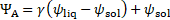
The buoyancy source term in Eq. (2) is described by the Boussinesq approximation, such that:
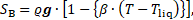
where ![]() is the gravity vector.
is the gravity vector.
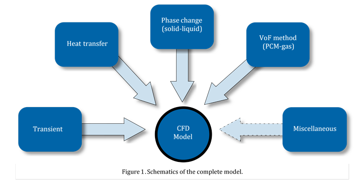
Figure 1 illustrates an overview of the complete model and is implemented in the open source FVM based CFD software OpenFOAM®. For the pressure-velocity coupling, the PIMPLE (PISO and SIMPLE) algorithm is employed. The VoF method is solved explicitly using a modified FCT (Flux Corrected Transport) method called MULES (Multidimensional Universal Limiter with Explicit Solution) and is based on the work of Zalesak [20] with an iterative calculation of the weighting factors [21]. A first order implicit Euler scheme is employed for the temporal discretization. For the gradient terms a second order Gauss linear scheme is applied. A variety of HRS (High Resolution Schemes) discretization schemes are used to solve the divergence terms of the equations.
3. Validation
3. 1. Stefan problem
The one-dimensional one-phase Stefan problem is a well-known transient heat transfer problem for directional solidification [1]. Figure 2 shows the schematic diagram of the problem.
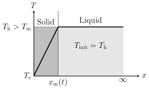
The fluid with
a melting point of ![]() = 882.15 K is used. The left and
right boundaries are kept at constant temperatures
= 882.15 K is used. The left and
right boundaries are kept at constant temperatures ![]() = 822.15 K (
= 822.15 K (![]() ) and
) and ![]() = 882.7 K (
= 882.7 K (![]() ) respectively. The initial
temperature of the system is
) respectively. The initial
temperature of the system is ![]() = 882.7 K and the thermophysical
properties of the fluid are tabulated in Table
1. The analytical solution for the determination of interface location
= 882.7 K and the thermophysical
properties of the fluid are tabulated in Table
1. The analytical solution for the determination of interface location ![]() at time t is given by:
at time t is given by:
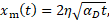
where ![]() is the thermal diffusivity, and
is the thermal diffusivity, and ![]() is
the non-linear eigenvalue and is determined by solving the below transcendental
equation using iterative methods.
is
the non-linear eigenvalue and is determined by solving the below transcendental
equation using iterative methods.
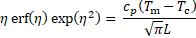
Table 1. Thermophysical properties of the fluid.
| Properties | Values |
| 1780 | |
| 1 x 10⁻³ | |
| 80 | |
| 1050 | |
| 339 |
In
the simulations a computational domain of size 150 mm x 2.5 mm (L ![]() B) is selected and discretized with
equidistant cell size of
B) is selected and discretized with
equidistant cell size of ![]() x = 0.5 mm, resulting in 1500 cells. The top and bottom boundaries are considered
as adiabatic; an empty[2] boundary condition is applied on the front and back boundaries of the domain.
x = 0.5 mm, resulting in 1500 cells. The top and bottom boundaries are considered
as adiabatic; an empty[2] boundary condition is applied on the front and back boundaries of the domain.
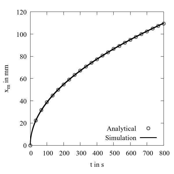
At time t = 0, solidification commences from the left boundary and continues to propagate towards the right boundary. Figure 3 shows a comparison of numerical simulation and analytical solution for the one-dimensional Stefan problem. The interface locations predicted by the simulation are in excellent agreement with the analytical solution.
3. 2. Melting of gallium
The melting of gallium in a rectangular enclosure is a well-documented solid-liquid phase change exp-eriment performed by Gau and Viskanta [22]. The computational domain is shown in Figure 4, the size of the domain is 88.9 mm x 63.5 mm and is divided into 42 x 32 hexahedral numerical cells.
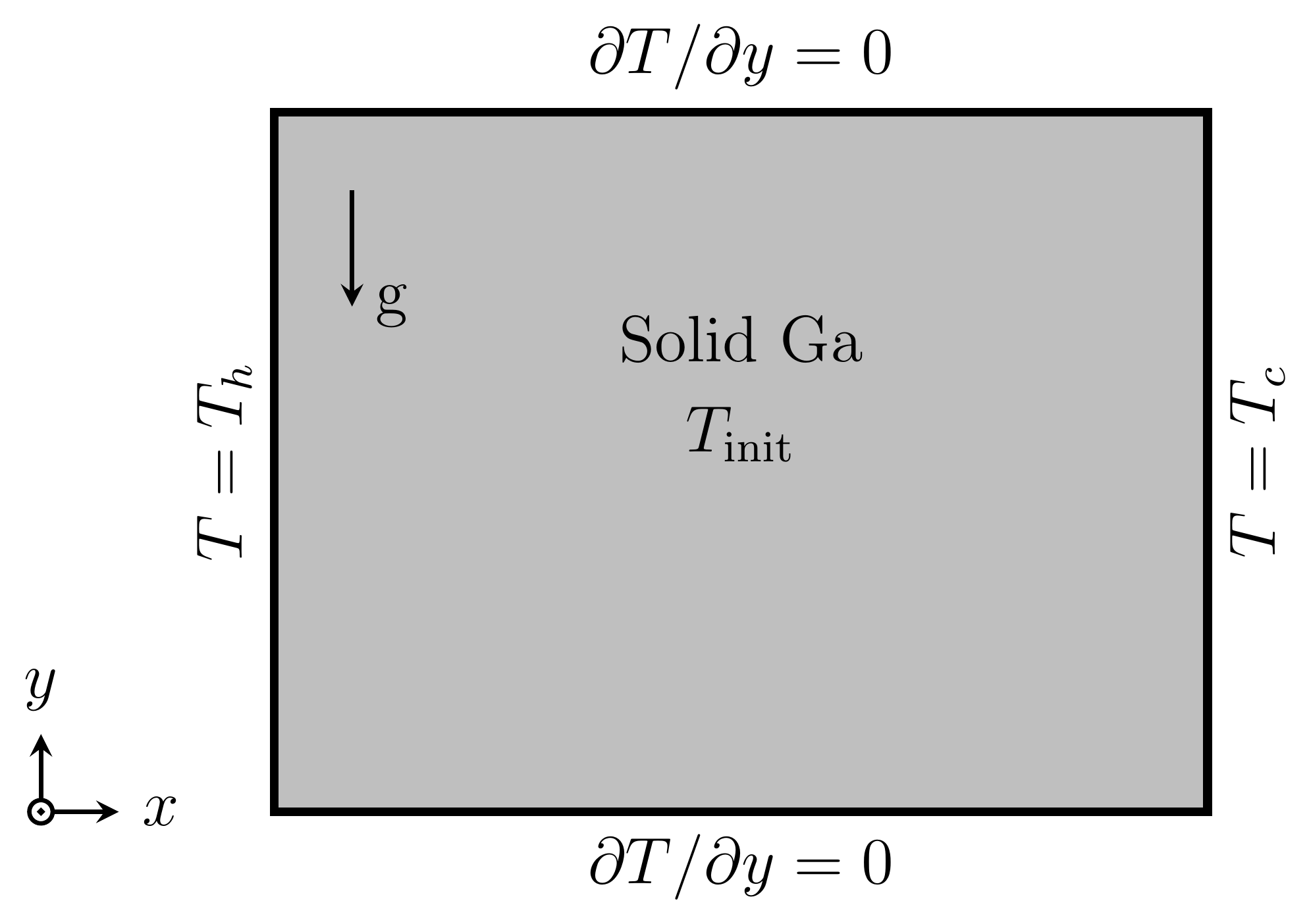
The left and
right walls are maintained at constant temperatures ![]() = 311.15 K,
= 311.15 K, ![]() = 301.45 K respectively. The top and
bottom walls are assumed to be adiabatic. The initial temperature of the system
is
= 301.45 K respectively. The top and
bottom walls are assumed to be adiabatic. The initial temperature of the system
is ![]() = 301.45 K. The thermophysical
properties of gallium used in the simulations are given in Table
2 Furthermore, the mushy zone constant C and the computational
constant ε in Eq. (13) are set to
1.6
= 301.45 K. The thermophysical
properties of gallium used in the simulations are given in Table
2 Furthermore, the mushy zone constant C and the computational
constant ε in Eq. (13) are set to
1.6 ![]() 106 kg m−3
s−1 and 1
106 kg m−3
s−1 and 1 ![]() 10−3 respectively,
see Brent et al [16].
10−3 respectively,
see Brent et al [16].
Table 2. Thermophysical properties of gallium.
| Properties | Values |
| 6093 | |
| 1.81 x 10⁻³ | |
| 32 | |
| 381.5 | |
| 80.160 | |
| 1.2 x 10⁻⁴ |
The temporal evolution of the melting front obtained from simulation exhibits good agreement with experiments of Gau and Viskanta [22] as shown in Figure 5.
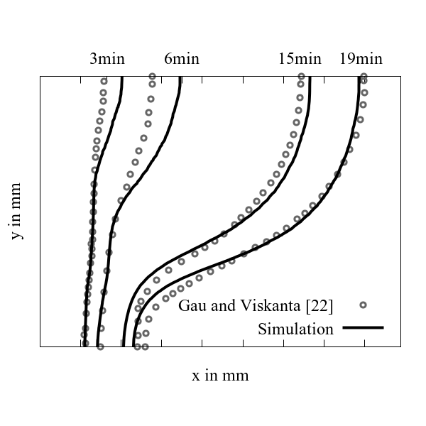
The slight deviations between the simulation and experiments can be explained as follows:
a. the melting fronts are obtained from two-dimensional simulation, whereas the experiments performed by Gau and Viskanta [22] were three-dimensional (for further information refer [5, 23]),
b. temperature independent thermophysical properties are used in the simulation,
c. the experiment was stopped multiple times and the melt was drained in order to track and record the melting front, which may have influenced the results.
3. 3. Free surface thermocapillary flow with phase change
A free surface thermocapillary flow
with phase change in a two-dimensional rectangular container under microgravity
conditions investigated by Tan et al. [13] is used for validation. For the sake
of validation, the source term ![]() in Eq. (8) is
resolved into the normal
in Eq. (8) is
resolved into the normal ![]() and the tangential
and the tangential ![]() components [13, 14, 24] and is expressed by:
components [13, 14, 24] and is expressed by:

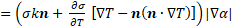
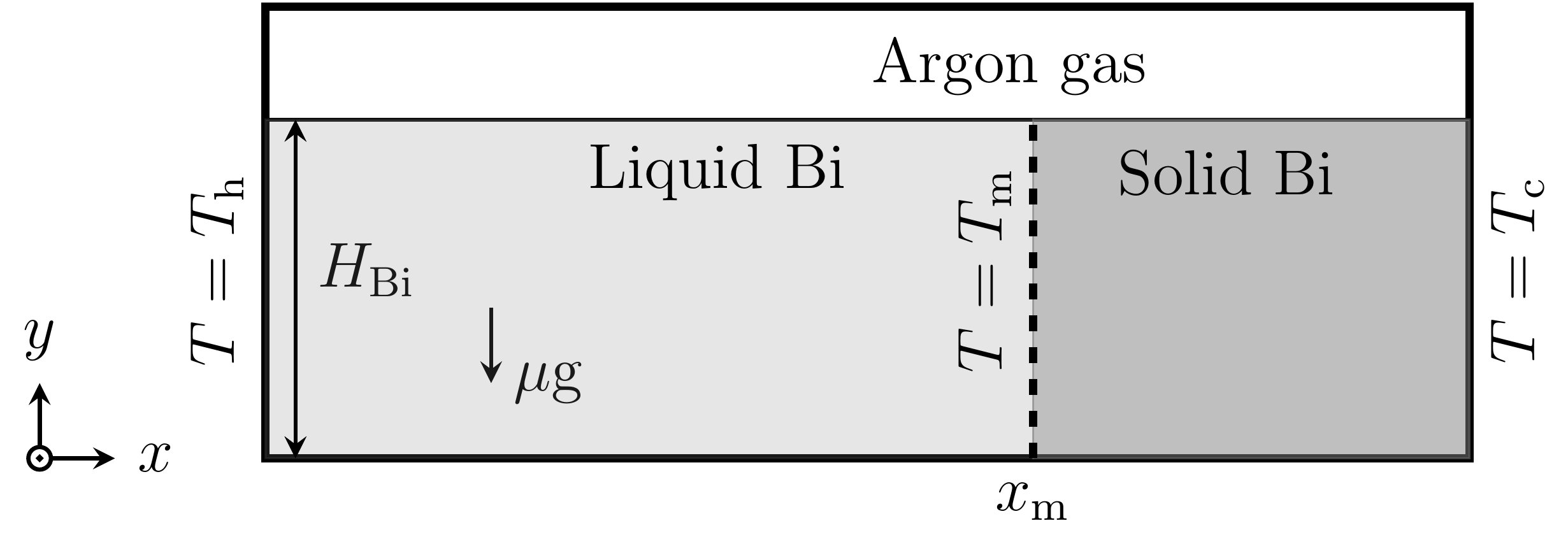
Figure 6 shows the computational domain of size 15 mm x 5 mm and is discretized into 140 x 62 hexahedral cells [13, 14]. The
bismuth melt is filled up to height ![]() = 4 mm and the rest is filled with
argon gas. The left and right walls are kept at constant temperatures
= 4 mm and the rest is filled with
argon gas. The left and right walls are kept at constant temperatures ![]() = 552.55 K and
= 552.55 K and ![]() = 540.55 K respectively. The top and
bottom walls are enforced with a linear temperature distribution from
= 540.55 K respectively. The top and
bottom walls are enforced with a linear temperature distribution from ![]() to
to ![]() , such that, the isoline of melting
temperature
, such that, the isoline of melting
temperature ![]() = 544.55 K is at a distance
= 544.55 K is at a distance ![]() from the left wall. The dimensionless
numbers corresponding to bismuth and argon gas are listed in Table
3[13]
from the left wall. The dimensionless
numbers corresponding to bismuth and argon gas are listed in Table
3[13]
Table 3. Dimensionless numbers.
| Symbol | Values |
| 244 | |
| 0.031 | |
| 0.0022 | |
| 0.033 | |
| 1.88 x 10⁻⁴ | |
| 0.019 |
where ![]() is the Marangoni number,
is the Marangoni number, ![]() Rayleigh number,
Rayleigh number, ![]() Capillary number,
Capillary number, ![]() Stefan number,
Stefan number, ![]() Biot number and
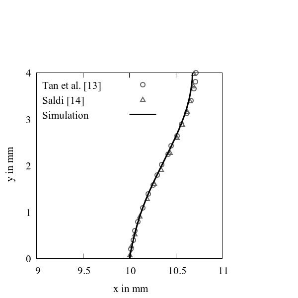
Biot number and ![]() Prandtl number. The comparison of
solid-liquid interface of the present work, the simulations by Tan et al. [13],
and the simulations by Saldi [14] is
shown in Figure
7. An excellent agreement is achieved in comparison with literature.
Prandtl number. The comparison of
solid-liquid interface of the present work, the simulations by Tan et al. [13],
and the simulations by Saldi [14] is
shown in Figure
7. An excellent agreement is achieved in comparison with literature.
4. Experimental setup
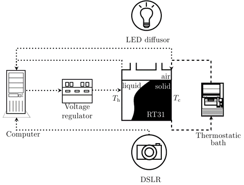
Experiments are conducted to further investigate the introduced model. Figure 8 illustrates the schematic of the experimental setup adapted from [11, 22, 26]. The domain consists of a square enclosure with inside dimensions of 50 mm x 50 mm x 50 mm made of Plexiglas. The left and right walls are made of aluminum plates which serve as heat source and heat sink respectively. A couple of multi-purpose riser pipes are screwed on the top wall of the enclosure which allows free flow of air to compensate for volume expansion/contraction during phase change. The enclosure is initially filled with paraffin wax (RT31) up to a height of 40 mm in liquid form through one of the riser pipes and is allowed to solidify for a certain period of time. All the walls are insulated except for the front and back walls. A DSLR camera is placed at an appropriate distance from the front wall to capture the sharp images of the temporal evolution of the melting front. A LED diffuser is placed at a suitable distance from the back wall in order to differentiate the solid and liquid phase during the melting process of the wax. Finally, all the images are processed and automated using ImageJ [25] for the evaluation of melting fronts and melt volume fraction of the paraffin wax.

5. Results and discussions
The thermophysical properties of RT26 to RT35 provided by the manufacturer [27] are comparable, the specific heat capacity and the thermal conductivity of the above mentioned PCMs are same and have uniform values for each (solid/liquid) phase. Shmueli et al. [10] compared their numerical results with experiments using the thermophysical properties provided by the manufacturer with a slightly varied thermal conductivities for solid and liquid phase. The thermophysical properties used in this study are adapted from the above literature and are tabulated in Table 4.
Table 4. Thermophysical properties used in CFD Simulations
| Properties | Rubitherm® RT31 | Air | |
| Solid | Liquid | ||
| 880 | 760 | 1.1885 | |
| - | 3.08 x 10⁻³ | 1.81 x 10⁻⁵ | |
| 0.24 | 0.15 | 0.0258 | |
| 2000 | 2000 | 1006 | |
| 160 | - | ||
| 7.6 x 10⁻⁴ | 3.38 x 10⁻³ |
The grid convergence study is
performed to investigate the influence of cell size on the melt fraction.
Different grid resolutions of 2D computational domain have been investigated,
from coarse (200 x 200 x 1) cells to fine (400 x 400 x 1) cells increased in steps of 25
cells in each x and y direction. A grid resolution of (275 x 275 x 1) is selected in this study. The
relative error of the melt fraction between the selected grid to the finest
grid resolution is less than 2%. An adaptive time stepping with Courant Number
(![]() ) of 0.75 is adopted.
) of 0.75 is adopted.
Figure
9 shows the experimental and numerical, temporal evolution of the
melting front at 15, 30, 45 and 60 min respectively, for the temperature at hot
and cold walls ![]() = 313.15 K and
= 313.15 K and ![]() = 295.15 K respectively. The liquid
paraffin close to the hot wall rises upwards and flow horizontally towards the
cold melting front, where it releases heat at the upper region of the solid
paraffin and descends along the cold melting front, thereby advancing the
melting front rapidly in the upper region than in the lower region. The
streamlines in the liquid paraffin shows that there is no movement approximately
at the center of the melt, this is because of the upwards and downwards flow of
liquid paraffin close to hot wall and cold melting front (indicated by solid
arrows in the bottom row of Figure
9). It is observed that the air flow above liquid paraffin also
progresses along with the melting front in a circular motion[3]. A
secondary air flow is also observed in the region above the solid paraffin. However,
the strength of this secondary air flow is minuscule. In the experiment it is
notable that the liquid paraffin-air interface is thicker than in simulations.
This is because of the contact angle between liquid paraffin-air interface and
the Plexiglas wall, which leads to the formation of meniscus near the Plexiglas
wall. Furthermore, the melting fronts in the simulation appear to be sharper
than in the experiment near the paraffin-air interface. This is because in
experiments the melting fronts are obtained by the evaluation of photographs
taken through front Plexiglas wall. Nevertheless, it is noteworthy to mention
that the surface tension effects are neglected during simulations.
= 295.15 K respectively. The liquid
paraffin close to the hot wall rises upwards and flow horizontally towards the
cold melting front, where it releases heat at the upper region of the solid
paraffin and descends along the cold melting front, thereby advancing the
melting front rapidly in the upper region than in the lower region. The
streamlines in the liquid paraffin shows that there is no movement approximately
at the center of the melt, this is because of the upwards and downwards flow of
liquid paraffin close to hot wall and cold melting front (indicated by solid
arrows in the bottom row of Figure
9). It is observed that the air flow above liquid paraffin also
progresses along with the melting front in a circular motion[3]. A
secondary air flow is also observed in the region above the solid paraffin. However,
the strength of this secondary air flow is minuscule. In the experiment it is
notable that the liquid paraffin-air interface is thicker than in simulations.
This is because of the contact angle between liquid paraffin-air interface and
the Plexiglas wall, which leads to the formation of meniscus near the Plexiglas
wall. Furthermore, the melting fronts in the simulation appear to be sharper
than in the experiment near the paraffin-air interface. This is because in
experiments the melting fronts are obtained by the evaluation of photographs
taken through front Plexiglas wall. Nevertheless, it is noteworthy to mention
that the surface tension effects are neglected during simulations.
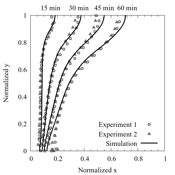
Figure 10 shows the comparison of melting fronts between experiments and simulation. The height of the liquid paraffin in the experimental domain varies due to the volume expansion during phase change. Therefore, for simplicity the temporal evolution of melting fronts has been normalized to the width of the experimental domain in x direction and to the height of the liquid paraffin in y direction. The melting fronts obtained by the numerical model are in good agreement with experiments.
However, the melting fronts at the lower region advances faster in experiments than in simulations, this is because the thermal conductivity of the Plexiglas walls also has an effect on the melting of the paraffin, however the influence of the Plexiglas walls is not considered during simulations.
6. Conclusions
In this study, a fundamental numerical model to tackle the solid-liquid phase change phenomena in the presence of gas phase has been investigated by means of well documented case studies in the literature and experimental validation. The model is based on the use of VoF approach to account for PCM and gas phase and enthalpy-porosity method to account for solid-liquid phase change in the PCM. The model has been validated using multiple references cases. The simulated results are in good agreement with the results described in the literature.
To further
investigate the limitations of the model, experiments with paraffin wax (RT31)
are conducted. Experiments are performed in a square enclosure partially filled
with paraffin wax in the presence of air. The left and right walls of the
enclosure are maintained at temperatures ![]() = 313.15 K and
= 313.15 K and ![]() = 295.15 K respectively, whereas the
remaining walls are assumed to be adiabatic. The temporal evolution of the melting
front obtained from simulation show a good agreement with the experiments. The
small discrepancies in the results can be accounted for, as follows:
= 295.15 K respectively, whereas the
remaining walls are assumed to be adiabatic. The temporal evolution of the melting
front obtained from simulation show a good agreement with the experiments. The
small discrepancies in the results can be accounted for, as follows:
- In experiments it is observed that the side Plexiglas walls also influence the melting phenomena within the enclosure, whereas in simulations these walls were not considered and are modeled as perfectly insulated.
- Temperature independent thermophysical properties are used in the simulations for PCM (solid/liquid) and gas phase.
- Only 2 dimensional simulations are carried out and the influence of the third dimension is not yet investigated.
- Finally, the errors in evaluation of photographs obtained from experiments due to volume expansion and surface tension effects.
Acknowledgements
The authors wish to acknowledge the Federal Ministry of Economic Affairs and Energy (BMWi), Germany for the financial support of MOTEVAS bearing project number 03ET1192B. Special thanks to the Computer Centre (URZ) of TU Bergakademie Freiberg for the HPC-Cluster support.
References
[1] D. M. Stefanescu, Science and Engineering of Casting Solidification. Second edition, Springer Science+Business Media, LLC, 2009.
[2] V. R. Voller, M. Cross and N. C. Markatos, “An enthalpy method for convection/diffusion phase change,” International Journal for Numerical Methods in Engineering, vol. 25, no. 1, pp. 271-284, 1987. View Article
[3] Henry Hu and Stavros A Argyropoulos, “Mathematical modelling of solidification and melting: a review,” Modelling and Simulation in Materials Science and Engineering, vol. 4, pp. 371-396, 1996. View Article
[4] F. Rösler and D. Brüggemann, “Shell-and-tube type latent heat thermal energy storage: numerical analysis and comparison with experiments,” Heat and Mass Transfer, vol. 47, no. 8, pp. 1027-1033, 2011. View Article
[5] A. Miehe, “Numerical investigation of horizontal twin-roll casting of the magnesium alloy AZ31,” Ph.D. dissertation, Technische Universität Bergakademie Freiberg, Freiberg, 2014.
[6] R. R. Kasibhatla, A. König-Haagen, F. Rösler, D. Brüggemann, “Numerical modelling of melting and settling of an encapsulated PCM using variable viscosity,” Heat and Mass Transfer, Springer, 2016. View Article
[7] König-Haagen, E. Franguet, E. Pernot, D. Brüggemann, “A comprehensive benchmark of fixed-grid methods for the modeling of melting,” International Journal of Thermal Sciences, vol. 118, pp. 69-103, 2017. View Article
[8] Hirt and B. Nichols, “Volume of Fluid (VOF) Method for the dynamics of Free Boundaries,” Journal of Computational Physics, vol. 39, pp. 201-225, 1981. View Article
[9] E. Assis, L. Katsman, G. Ziskind, R. Letan, “Numerical and experimental study of melting in a spherical shell,” International Journal of Heat and Mass Transfer, vol. 50, pp. 1790-1804, 2007. View Article
[10] H. Shmueli, G. Ziskind, R. Letan, “Melting in a vertical cylindrical tube: Numerical investigation and comparison with experiments,” International Journal of Heat and Mass Transfer, vol. 53, pp. 4082-4091, 2010. View Article
[11] F. Rösler, “Modellierung und Simulation der Phasenwechselvorgänge in makroverkapselten latenten thermischen Speichern,” Ph.D. dissertation, Universität Bayreuth, 2014. (German)
[12] R. R. Kasibhatla, A. König-Haagen, D. Brüggemann, “Numerical modelling of wetting phenomena during melting of PCM,” Procedia Engineering, vol. 157, pp. 139-147, 2016. View Article
[13] L. H. Tan, S. S. Leong, T. J. Barber and E. Leonardi, “Simulation of solidification with Marangoni effects using a multiphase approach,” Progress in Computational Fluid Dynamics, vol. 6, no. 6, pp. 305-313, 2006.
[14] Z. S. Saldi, “Marangoni driven free surface flows in liquid weld pools,” Ph.D. dissertation, Technische Universiteit Delft, Delft, 2012.
[15] O. Richter, J. Turnow, N. Kornev, E. Hassel, “Numerical simulation of casting processes: coupled mould filling and solidification using VOF and enthalpy-porosity method,” Heat Mass Transfer, vol. 43, pp. 1957-1969, 2017. View Article
[16] A. D. Brent, V. R. Voller, and K. J. Reid, “Enthalpy-porosity technique for modeling convection-diffusion phase change: Application to the melting of a pure metal,” Numerical Heat Transfer, vol. 13, pp. 297-318, 1988. View Article
[17] V. R. Voller and C. Prakash, “A fixed grid numerical modelling methodology for convection-diffusion mushy region phase change problems,” International Journal of Heat and Mass Transfer, vol. 30, no. 8, pp. 1709-1719, 1987. View Article
[18] H. Rusche, “Computational fluid dynamics of dispersed two-phase flows at high phase fractions,” Ph.D. thesis, Imperial College of Science, Technology and Medicine, London, 2002.
[19] J. U. Brackbill, D. B. Kothe and C. Zemach, “A Continuum Method for Modeling Surface Tension,” Journal of Computational Physics, vol. 100, pp. 335-354, 1992. View Article
[20] S. T. Zalesak, “Fully multidimensional Flux-Corrected Transport Algorithms for Fluids,” Journal of Computational Physics, vol. 31, pp. 335-362, 1979. View Article
[21] S. M. Damian, “An extended mixture model for the simultaneous treatment of short and long scale interfaces,” Ph.D. thesis, Universidad Nacional del Litoral, 2013.
[22] C. Gau and R. Viskanta, “Melting and Solidification of a Pure Metal on a Vertical Wall,” Journal of Heat Transfer, vol. 108, pp. 174-181, 1986. View Article
[23] K. Wittig and P. A. Nikrityuk, “Three-dimensionality of fluid flow in the benchmark experiment for a pure metal melting on a vertical wall,” in IOP conference series: Material science and engineering, vol. 27, 2012. View Article
[24] T. Yamamoto, Y. Okano and S. Dost, “Validation of the S-CLSVOF method with the density-scaled balanced continuum surface force model in multiphase systems coupled with thermocapillary flows,” International Journal for Numerical Methods in Fluids, vol. 83, pp. 223-244, 2017. View Article
[25] ImageJ, [Online]. Available: https://imagej.nih.gov/ij/index.html
[26] Y. Wang, A. Amiri, K. Vafai, “An experimental investigation of the melting process in a rectangular enclosure,” International Journal of Heat and Mass Transfer, vol. 42, pp. 3659-3672, 1999. View Article
[27] Rubitherm Technologies GmbH, [Online]. Available: https://www.rubitherm.eu/en/index.php/productcategory/organische-pcm-rt