Journal of Fluid Flow, Heat and Mass Transfer (JFFHMT)
ISSN: 2368-6111

Volume 5 - Year 2018 - Pages 53-70
DOI: 10.11159/jffhmt.2018.006
Analysis of the Drift Flux in Two-Phase Gas-Liquid Slug-Flow along Horizontal and Inclined Pipelines through Experimental (Non)-Newtonian and CFD Newtonian Approaches
Paula D. Pico1, Juan P. Valdés1, Nicolás Ratkovich1, Eduardo Pereyra2
1Department of Chemical Engineering, Universidad de los Andes Carrera 1 # 18a-12 Bogota, Colombia
pd.pico10@uniandes.edu.co; jp.valdes10@uniandes.edu.co; n.rios262@uniandes.edu.co
2McDougall School of Petroleum Engineering, The University of Tulsa
Tulsa, OK 74104, United States
eduardo-pereyra@utulsa.edu
Abstract - The objective of this study is to analyze the influence of the physical properties of Newtonian and Non-Newtonian fluids, such as density, effective viscosity and surface tension, as well as operational parameters of the piping, such as diameter, length and angle of inclination, on the drift velocity for twophase gas-liquid flow. This study comprises a Computational Fluid Dynamics (CFD) approach for Newtonian fluids and an experimental approach for both, Newtonian and NonNewtonian fluids. The simulation model consisted of half a section of a circular pipe with a symmetry plane. This model was calibrated through a mesh independence test, which considered experimental and literature data as benchmarking values for both low and high viscosity Newtonian fluids. The results obtained through the CFD model showed good agreement with the experimental data gathered for the present study, keeping the experimental deviations under 10% for most (roughly 95%) of the cases considered. The relationship between the Froude number (Fr) and the Viscosity number (Nvis) was studied and an inverse exponential tendency was found for all the parameters and fluids tested, which agrees with the models proposed in literature. The data gathered for all fluids on the drift velocity’s behavior against operational parameters such as length, diameter and inclination, showed the influence of the governing forces for each case based on dimensionless analysis using Eötvös (Eö) and Reynolds (Re) numbers. For dominant capillary or viscous forces on the system, the drift velocity changed with the variation of these parameters. However, it was found that for dominant inertial and gravitational forces, the drift velocity maintained a constant value regardless of the operational settings. Finally, it was observed that the rheological nature found for the Non-Newtonian fluids has a significant influence on the drift velocity’s behavior, deviating its patterns from the Newtonian fluids as the effective viscosity changed.
Keywords: Drift Flux, CFD, Froude Number, Viscosity Number, Two-phase.
© Copyright 2018 Authors - This is an Open Access article published under the Creative Commons Attribution License terms Creative Commons Attribution License terms. Unrestricted use, distribution, and reproduction in any medium are permitted, provided the original work is properly cited.
Date Received: 2018-05-07
Date Accepted: 2018-09-05
Date Published: 2018-10-01
Nomenclature
- vT - Translational Velocity (m/s)
- Co - Distribution parameter or flow coefficient
- vm - Velocity of the total mixture (m/s)
- vd - Drift Velocity (m/s)
- nP - Flow behavior index
- KP
- Flow consistency index

 – Effective viscosity (Pa*s)
- D - Diameter of pipe (m)
 - Shear rate
(1/s)
- Shear rate
(1/s)- μ - Dynamic Viscosity (Pa* s) (subscript L corresponds to liquid phase)
- ρ - Density (kg/m3) (subscript g and L stands for gas and liquid phase respectively)
- σ - Surface Tension (N /m)
 – Angle of inclination (deg)
- Fr - Froude Number
- Eo - Eötvös Number
- Nvis - Viscosity Number
- Re - Reynolds Number
 - kth-phase volumetric fraction
(subscript g and L stands for gas and liquid phase respectively)
- kth-phase volumetric fraction
(subscript g and L stands for gas and liquid phase respectively)
- P – Pressure (Pa)
 – Velocity (vectorial notation) (m/s)
 – Mean
velocity (vectorial notation) (m/s)
– Mean
velocity (vectorial notation) (m/s) – Turbulent velocity (vectorial notation) (m/s)
 - Gravity (vectorial notation) (m/s2)
 - Gravity (m/s2)
 – Volumetric
forces at the interface due to surface tension (N/m3)
– Volumetric
forces at the interface due to surface tension (N/m3)- vg /vL – Velocity of the gas / liquid phase (m/s)
- k – Kinetic energy
 – Turbulent
rate of dissipation (subscript 0 stands for ambient turbulence value)
– Turbulent
rate of dissipation (subscript 0 stands for ambient turbulence value)- μT – Turbulent Viscosity
 - turbulent model coefficients
 – Production terms for the turbulent model
 – Damping function
 – Source terms for the turbulent model
 – Distance
from the wall pipe
– Distance
from the wall pipe – Dimensionless wall distance
 – Friction velocity
 – Wall shear stress
 – Freestream velocity
1. Introduction
In the past few decades, all efforts of the oil and gas industry have shifted towards the extraction, transportation and refinement of heavier oils, as they represent nearly 70% of the actual available reserves of crude oil [1]. In the past, all crude oil extraction was focused almost exclusively on light oil reserves, as the exploration and drilling technologies were only available for low-viscosity fluids, which meant lesser costs associated with its production. However, these reserves were depleted, which led to the need of increasing and improving extraction technologies for high density and viscosity hydrocarbons. Non-Newtonian fluids are also commonly encountered in the upstream petroleum industry as waxy crude oils, gelled oils, drilling muds, fracturing fluids (for non-conventional oil and gas resources) and slurries [2]. Therefore, it became of great interest to extend the applicability range and improve the existing knowledge on multiphase flow models to consider liquid phases with high viscosities and Non-Newtonian rheological behavior.
Currently,
most of the existing multiphase flow models used to predict important operational
parameters, such as translational velocity of the oil mixture or pressure drop
along the pipeline, are only accurate for low viscosity fluids (<0.01 Pa*s)
and have a wide range of limitations to be properly applied. Consequently,
these models do not account for the effects of high viscosity or apparent
viscosity (for Non-Newtonian fluids) and cannot be generalized for various
operational conditions and neither can be unified for variations on fluid
properties. Moreover, few different approaches can be found in literature for
slug flow pattern modelling and they present incomplete or narrow-scoped
correlations to estimate important parameters such as the drift flux. Various
experimental studies such as Gregory & Scott (1969) in a fully developed
slug flow CO2-water cocurrent system [3], and Heywood
& Richardson (1979) in a water-air system using ![]() -ray
absorption [4], initially
considered a null drift velocity in the estimation of the translational
velocity of the slug unit in horizontal pipes. Both studies estimate this
velocity as a function of the “no-slip” velocity alone, which corresponds to
the total volumetric flowrate of the mixture divided by the cross sectional
area of the pipe [4]. Similarly,
analytical studies from Duckler & Hubbard (1975) [5] in
horizontal and near horizontal tubes modelled the rate of advance of the slug
(translational velocity) as a function of the mean velocity of the fluid
relative to the pipe wall and the rate of buildup at the front of the slug due
to film pickup. Therefore, the drift velocity component was not considered in
the calculation, given that gravity cannot act in the horizontal direction.
-ray
absorption [4], initially
considered a null drift velocity in the estimation of the translational
velocity of the slug unit in horizontal pipes. Both studies estimate this
velocity as a function of the “no-slip” velocity alone, which corresponds to
the total volumetric flowrate of the mixture divided by the cross sectional
area of the pipe [4]. Similarly,
analytical studies from Duckler & Hubbard (1975) [5] in
horizontal and near horizontal tubes modelled the rate of advance of the slug
(translational velocity) as a function of the mean velocity of the fluid
relative to the pipe wall and the rate of buildup at the front of the slug due
to film pickup. Therefore, the drift velocity component was not considered in
the calculation, given that gravity cannot act in the horizontal direction.
However, it has been demonstrated analytically and experimentally that the drift velocity component is not zero, even for a horizontal arrangement of the pipeline. Benjamin (1968) based his work on the inviscid potential flow theory to determine the drift velocity, suggesting that, in horizontal slug flow, it is the same as the velocity of penetration of a gas when the liquid is drained out of the pipe [6]. Weber (1981) showed through a balance of forces on the bubble and Young-Laplace equation that drift velocity is not always zero for horizontal flow but has a limiting Eo value (Eo=12) which determines if the bubble has motion [7].
Bendiksen (1984) [8] and Weber et al. (1986) [9] experimentally studied the influence of the angle of inclination and pipe diameter on the drift velocity considering a dimensionless analysis through Froude, Reynolds and Eötvös numbers. Bendiksen (1984) found that, for any inclination, a critical liquid velocity is reached where the bubble turns and propagates faster than the average liquid. Moreover, experimental data for all inclinations supported the existence of a drift velocity occurring due to buoyancy or level effects which affected the bubble´s propagation rate [8]. Weber et al. (1986) found that the drift velocity presents a broad maximum for angles of inclination between 30° and 60°. Additionally, Eo limiting values were tested experimentally and consistent results were observed with the author´s previous theoretical studies. Further analysis showed that the drift velocity was very sensitive in the near horizontal region for sufficiently large Eo numbers, which correspond to bigger pipe diameters and/or fluids with smaller surface tension.
More recently, Gockal (2008) focused his study on the effect of high viscosity oils for horizontal two-phase flow in pipelines. Gockal noted a considerable difference between low and high viscosity fluids. Intermittent slug flow and elongated bubbles was the dominant flow pattern generated and concluded that for decreasing Reynolds numbers, the bubble velocity decreases [10]. Losi et al. (2016) evaluated the effect of viscosity and inclinations in the drift velocity of a penetrating air bubble. It was found that the drift velocity is not constant along the pipe for horizontal flow, given that the viscosity slows down the propagation of the bubble along the pipe [11].
Several
researchers have recently adopted a Computational Fluid Dynamics (CFD) scope on
the study of multiphase flow in order to validate and complement previous
experimental advancements. One of the earliest uses of CFD for drift flux
prediction was done by Andreussi and Bonizzi (2009) with the commercial
software FLUENT [12].
These authors used the VOF approximation to model the two-phase system and studied
the motion of the bubble along the pipe and the influence of the fluid´s
viscosity on the drift velocity. They found that higher viscosities tend to
cause a decrease on the drift velocity along the pipe´s length. Barcelo et al.
(2010) developed a CFD model in Open FOAM based on the drift flux model to
analyze the behaviour of oil-water separators, considering an Eulerian
multiphase approach and a ![]() turbulent turbulence model[13].
Ramdin and Henkes (2012) proposed the analysis of varying viscosity and surface
tension through the calculation of the Froude number and Eötvös number[14].
This work used commercial CFD code from FLUENT, along with the VOF
approximation for two-phase modelling and found that the drift velocity decreases
with decreasing Eötvös number and that velocity decreases in time as the bubble
travels through the pipe.
turbulent turbulence model[13].
Ramdin and Henkes (2012) proposed the analysis of varying viscosity and surface
tension through the calculation of the Froude number and Eötvös number[14].
This work used commercial CFD code from FLUENT, along with the VOF
approximation for two-phase modelling and found that the drift velocity decreases
with decreasing Eötvös number and that velocity decreases in time as the bubble
travels through the pipe.
More recently, Kroes and Henkes (2014) studied the drift velocity of elongated gas bubbles in liquid-filled pipelines using FLUENT (ANSYS 14), obtaining good agreement with the inviscid analytical solution and with experimental data [15]. The data taken by this study helped develop various correlations to replicate, and further validate, previous experimental findings on the time-dependent behaviour of drift velocity as a function of liquid viscosity. Lu (2015) performed an experimental and computational investigation on horizontal gas-liquid two phase slug-flow, in order to describe the slug initiation, growth and collapse along the pipeline [16]. Six CFD codes were used throughout this research (STAR-CD, CFX, FLUENT, LedaFlow, TRIOMPH, TransAT), with the objective of studying convergence methods in terms of accuracy and fast processing. Similarly, Sanderse et al. (2015) simulated elongated bubbles travelling through a channel using the two-phase model and the CFD software FLUENT [17]. This research had the main objective of predicting the bubble drift velocity and the pressure variation along the channel. The results obtained for the Benjamin bubble were validated against a 2D CFD solution for inviscid flow.
Experimentally, very few studies can be found on Non-Newtonian fluids related with multiphase systems. Bishop (1986) studied a Non-Newtonian liquid gas system for stratified flow on horizontal tubes [18]. It was found that for very low liquid velocities the flow pattern observed was non-uniform and the two-phase drag reduction predicted by Heywood-Charles model was not reached due to a transition to semi-slug flow. Iluta (1996) carried out an experimental investigation to determine the influence of the flow consistency index for Non-Newtonian fluids on important operational parameters such as pressure drop and liquid holdup for two-phase flow in fixed beds [19] Good agreement was found between the predicted and measured values of the two-phase pressure drop and liquid holdup for the gas-Non Newtonian systems considering correlations for Newtonian fluids. More recently, Dziubinski (2004) developed a flow pattern map for two-phase Non-Newtonian liquid-gas flow in a vertical pipe from an experimental approach [20]. It was observed that the same flow structures appear for multiphase mixtures, regardless of a Newtonian or Non-Newtonian liquid phase. Additionally, it was concluded that Non-Newtonian characteristics of liquids has a negligible effect on the type of two-phase flow structure.
As can be noted from the state of the art previously presented, there is a considerable amount of information regarding the influence of several individual parameters on the behaviour of the drift velocity along pipelines. However, a comprehensive experimental and CFD study that unifies the effect of all parameters analyzed in previous studies is yet to be done. Subsequently, the present study seeks to analyze simultaneously the influence of the pipe diameter, length, and inclination angle, as well as the fluid’s density, surface tension and rheological behaviour on the drift velocity´s behavior along pipelines considering two-phase, gas-liquid slug flow. This will be performed through a quantitative and qualitative dimensionless analysis between Froude number (Fr), Viscosity number (Nvis), Reynolds number (Re) and Eötvös number (Eö) which involves simultaneously all parameters previously mentioned. It is important to clarify that the CFD approach was only considered for Newtonian fluids, whilst the experimental procedure was carried out for Newtonian and Non-Newtonian fluids.
1.1. Translational Velocity
The term translational velocity for multiphase flow studies is defined as the velocity at which a slug unit travels [1]. The slug unit refers to the combination of gas bubbles travelling along with alternating liquid slugs, generating the commonly known slug flow pattern. This velocity is usually expressed in terms of the velocity component of the total mixture multiplied by a flow coefficient or distribution parameter and the drift velocity. The initial expression for the translational velocity of the slug unit was proposed by Nicklin et al. (1962) [21]< as shown in Eq (1).

The
distribution parameter ![]() is defined as the approximate ratio between the
maximum and the average velocity of the slug unit considering a fully developed
velocity profile. This ratio is determined from the assumption that the
propagation velocity of the gas bubble follows the maximum local liquid
velocity in front of the nose tip as proposed by Kroes & Henkes (2014) [15]. For laminar
flow, the flow coefficient is approximately 2 as estimated by Nicklin et al.
(1962) [21] and for
turbulent flow the value of the flow coefficient is estimated to be 1.2 as
given by Wallis (1969) [22]. Current
multiphase flow models use the translational velocity to understand the
behavior of the mixture travelling along the pipeline. To properly calculate
this parameter, it is important to consider the contribution made by the drift
velocity.
is defined as the approximate ratio between the
maximum and the average velocity of the slug unit considering a fully developed
velocity profile. This ratio is determined from the assumption that the
propagation velocity of the gas bubble follows the maximum local liquid
velocity in front of the nose tip as proposed by Kroes & Henkes (2014) [15]. For laminar
flow, the flow coefficient is approximately 2 as estimated by Nicklin et al.
(1962) [21] and for
turbulent flow the value of the flow coefficient is estimated to be 1.2 as
given by Wallis (1969) [22]. Current
multiphase flow models use the translational velocity to understand the
behavior of the mixture travelling along the pipeline. To properly calculate
this parameter, it is important to consider the contribution made by the drift
velocity.
1.2. Drift Velocity
The drift
flux parameter refers to the velocity at which the gaseous phase travels and
penetrates through the stagnant liquid phase within the pipe. The drift flux model treats the mixture as a single
pseudo-fluid rather than two separate phases, yet it considers the interface
slip and interactions between both phases [23].
Consequently, the drift flux model consists of only four field differential
equations from the original six, eliminating one energy and one momentum
equation. Given this, it is important to mention that the drift flux model
replaces dynamic interactions (relative motion and energy difference) between
phases given by the field functions with constitutive laws which provide
relative velocity between phases (kinematic relation between phases) and
thermal interaction between phases [24].The
model is characterized through four dimensionless parameters, the ![]() ,
, ![]() ,
, ![]() and
and ![]() numbers. The definitions of these
dimensionless numbers, according to Moreiras (2014) [1],
are given as follows:
numbers. The definitions of these
dimensionless numbers, according to Moreiras (2014) [1],
are given as follows:
The differential equations by which the drift flux is modelled include continuity for one phase (usually the gaseous phase) and three conservation equations for the mixture which include continuity, momentum and energy [24]. Based on the formulation mentioned, the drift-flux model follows the standard approach used to analyze the dynamics of a mixture of gases or miscible liquids. Therefore, this model is generally well accepted for mixtures where the dynamics of both phases are closely coupled and share a well-defined interface surface region.
This model takes into account the effects of non-uniform velocity and void fraction profiles, as well as the effect of the local relative velocity between the phases [25]. Its application has resulted very successful in several engineering problems related with forced convection systems involving two-phase flow dynamics. The drift flux model however results much simpler in its formulation in comparison to other two-fluid models due to several considerable assumptions that must be considered, one of them being the pseudo-fluid treatment for the two-phase mixture. On the other hand, in the application of engineering problems, these assumptions become very useful as they allow detailed analysis of two-phase flow behavior to be carried out with less difficulty. In two-phase flow dynamics, information required for engineering problems usually comes from the response of the mixture as a whole, rather than two separate responses of each phase [24].
The drift flux model, despite being less rigorous than other more detailed two-phase flow models, is extremely important since it allows to properly predict and identify the physical structure of the flow in a relatively simple way [25]. Due to the importance of parameters such as the mixture velocity or pressure drop in the Oil and Gas (O&G) industry, several efforts have been made to improve the existing knowledge on drift velocity, and therefore improving the tools available to predict accurately multiphase flow behavior in pipelines.
2. Materials and Methods
The following section is divided in two main subsections: the experimental study carried out to complement and validate the information obtained from the computational simulations and the CFD modelling proposed for the simulations, which includes the spatial discretization constructed for the mesh and the physical models considered.
2.1. Experimental Procedure
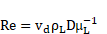
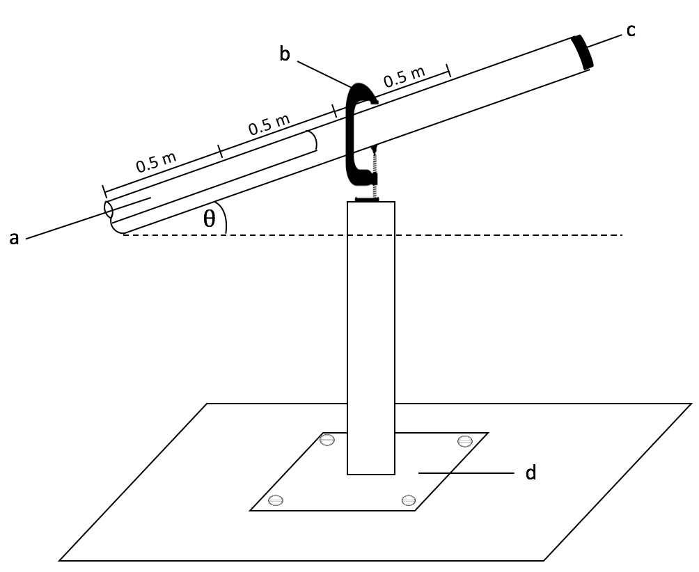
The drift velocity was estimated experimentally by measuring the time it takes for the gas bubble to travel across a designated distance. The apparatus used consisted of a set of 3 acrylic pipes with equal longitudinal dimensions and varying diameters. All pipes were 2 meters long and had inner diameters of 17, 24 and 44 mm, respectively. The lower end of the pipe was fitted with a plug, which was held by a highly resistant insulating tape to facilitate the filling process and guarantee that the plug would not yield under the fluid´s weight. The pipe was set at four different inclination angles (10°, 20°, 30° and 40°) with an adjusting metallic clamp and held horizontally on a previously calibrated stand at zero degrees of inclination with the upper end set above of a disposal bucket and fitted with an easily removable plug.
Initially, the pipe is fitted with a non-removable plug at one end, filled with the test fluid and closed with a second plug while it is accommodated to the desired angle of inclination. Once the pipe is set, the second plug is released, which causes the fluid to drain and the bubble to enter the pipe and displace the liquid. The entrance of the bubble occurs due to gravitational potential energy generated from the hydrostatic pressure difference between the initial and final segment of the bubble nose [26]. The measuring procedure consisted of one calibrated chronometer set to start as soon as the upper end plug was released. Once the bubble tip reached the marks previously placed on the tubes, the chronometer would be paused, and time would be recorded. All acrylic pipes were marked with the distances considered for the measurements, these distances being 0.5, 1 and 1.5 m for low viscosity fluids, and 0.2, 0.4, 0.5, 0.6, 0.8, 1 and 1.5m for high viscosity Newtonian and Non-Newtonian fluids. A general diagram of the experimental facility is shown in Fig. 1.
The properties of the studied fluids were measured in the facilities of the Universidad de los Andes and are summarized in Table 1. The rheological behavior was measured using a TA Instruments Discovery Hybrid Rheometer-1 with a logarithmic shear rate sweep at a constant temperature of 25°C. A smooth stainless-steel Peltier 20mm plate geometry (for the last three fluids in Table 1 which exhibit higher viscosities) and a concentric conical cylinder geometry of 28mm diameter and 42mm of length (for the rest of the fluids) were used for the measurements. The fluids which presented small or no variation of the viscosity for the different shear rates tested were considered as Newtonian for the present study. As for the surface tension measures, these were taken by a dynamic contact angle tensiometer using the Wilhelmy plate method, which consists of a thin plate which is oriented perpendicular to the interface between the fluids of interest (in this case in the air-fluid interface). The force exerted by the plate as it is wetted is then measured and used to estimate the surface tension with the Wilhelmy equation. The density was measured through the use of a simple metallic pycnometer of known internal volume and weight. The pycnometer was filled with the test fluid and its new weight recorded in order to determine the fluid´s weight and hence calculate its density.
The
Non-Newtonian fluids were modelled through a power law model to describe their
rheological behavior [27]. As seen in Table 1, all
Non-Newtonian fluids tested follow a pseudo-plastic behavior with a flow
behavior index of ![]() <1. In order to calculate the effective
viscosity appropriately, the shear rate’s definition was taken from Darby
(2001) [28] as shown in
Eq. (6).
<1. In order to calculate the effective
viscosity appropriately, the shear rate’s definition was taken from Darby
(2001) [28] as shown in
Eq. (6).
Table 1. Measured properties of the fluids tested at 0.74 bar and 25 °C.
| Fluid | Newtonian | Non-Newtonian | |||
| Water | 1000 | 0.001 | 72.00 | X | |
| IsoparL Oil | 762.29 | 0.001 | 24.00 | X | |
| Mineral Oil | 863.104 | 0.031 | 32.00 | X | |
| Sunflower Oil | 899.19 | 0.055 | 33.00 | X | |
| Olive Oil | 924.391 | 0.061 | 32.00 | X | |
| Hydraulic Oil | 893.122 | 0.092 | 31.00 | X | |
| Maple Syrup | 1380.374 | 0.572 | 50.00 | X | |
| Honey | 1468.687 | 7.105 | 54.00 | X | |
| Shampoo | 1001.46 | Kp=8.2122 ; np=0.716 | 21.00 | X | |
| Chocolate Syrup | 1333.391 | Kp=26.597 ; np=0.319 |
32.00 | X |
2.2. CFD Modelling
The CFD simulations were performed in the commercial software STAR-CCM+ v12.04.011 considering a finite volume approach. The geometry was generated through the STAR-CCM+ CAD tool.
2.2.1. Geometry Modelling and Mesh Generation
The geometry that was simulated consisted of half a circular pipe with a symmetry plane and a single outlet face, as shown in Fig 2 (a). The spatial discretization of the pipeline was constructed considering a polyhedral volume meshing model and a prism layer model. The polyhedral mesh guarantees that each cell has a large number of immediate neighbouring cells of which the software can obtain information and use linear shape functions, resulting in a better approximation of the gradients, lower skewness angles and a more accurate flux calculation when compared to a tetrahedral mesh [29].
Additionally, a polyhedral shape allows a higher probability of finding a direction within the cell that aligns with the direction of the flow [29]. Moreover, according to several practical studies [30], polyhedral meshes need approximately four times fewer cells to achieve the same level of accuracy when compared to a tetrahedral mesh [29].
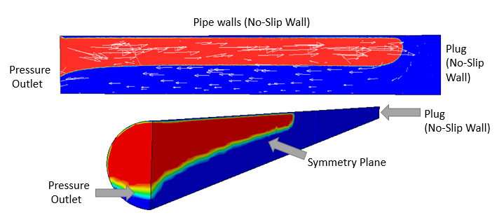
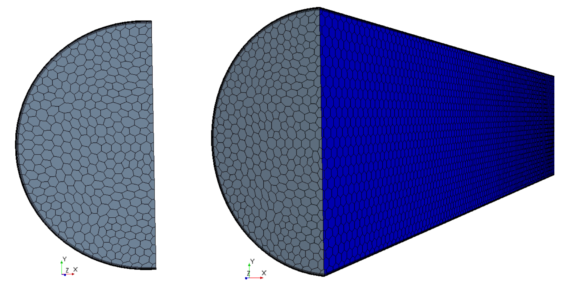
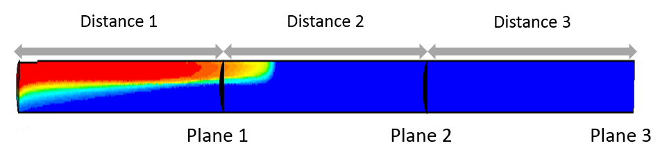
Figure 2. (a) Boundary conditions, bubble domain is colored red and liquid domain is colored blue. (b) Polyhedral mesh generated on the pipeline. (c) Spatial locations of the reference planes for the calculation of the CFD drift velocity.
The prism layer model allows the accurate resolution of near-wall flow features related to the boundary layer and the law of the wall on turbulent flow regimes [31]. These calculations are achieved by constructing prismatic orthogonal cells near a wall surface. This model additionally reduces a particular numerical discretization error near the wall boundary known as numerical diffusion. For this research, the number of prism layers was set to 8 with a constant growth rate of 1.5 to guarantee appropriate near-wall results. The prism layer total thickness was fixed as 24% relative to the base size of the volume mesh to assure an adequate value of the dimensionless wall distance (refer to Sub-section 2.2.3 for a detailed analysis of this parameter). The final settings considered for the mesh construction are described in section 3.1 with the mesh independence test results.
2.2.2. Physical Models Specification
The physics chosen to model the two-phase flow behavior on the current investigation was the Eulerian-Eulerian approach, implemented through the VOF model developed by Hirt and Nichols [32]. This model consists of a single set of momentum and turbulence equations for the continuous phase and an additional transport equation for the dispersed phase based on its volumetric fraction[33]. The VOF model has been previously used in other applications from the O&G industry such as design of skim tanks for oil removal [34], oil spilling [35] and sloshing[36].
The VOF model allows a good interpretation of the physical phenomenon studied for the drift velocity, given that it considers appropriately the phase to phase interaction by modelling the effects of surface tension on the free surface through the Continuum Surface Force (CSF) model [33]. It also allows a tracking of the interface by solving a continuity equation for the volume fraction of the dispersed phase[37]. These aspects guarantee the formation of a well defined free surface region where the motion of the bubble can be appropriately captured. The High-Resolution Interface-Capturing (HRIC) scheme is used, allowing a sharper interface between the fluids by reducing the numerical diffusion [38]. With this VOF model, it is possible to estimate correctly the velocity at which the bubble will travel along the pipeline through the stagnant liquid phase as it considers the interacting surface tension forces and generates an appropriate free surface region/interface.
Additionally, this model allows the consideration of the mixture as a single pseudo-fluid rather than two separate phases by solving one mass-averaged momentum equation for the whole domain and one equation of continuity per phase to track the change on the interface as seen in Eqs (7) - (8)[38].
Therefore, any interface/mixture
parameters and variables such as density and viscosity (Minterphase)
can be calculated through interpolation of each phase value (Mg and
ML for gas and liquid phase properties respectively) using the
volume fraction ![]() of each phase per cell, as seen in Eqs (9) - (10)[37],[38].
of each phase per cell, as seen in Eqs (9) - (10)[37],[38].

The VOF model was selected because, for this application, it is especially useful for locating and accurately tracking the free surface region where the interface is located by calculating the volume fraction of the secondary phase on each cell [37]. Additionally, it considers the effect of surface tension forces on the motion of the bubble through the CSF model as mentioned previously. However, this model causes the appearance of parasitic currents [39]. These are unphyisical currents which are generated due to the discontinuity of the domain in regions such as the interface [33]. These solution discontinuities across the free surface can cause discretization errors which end up forming parasitic currents. In order to reduce these currents, especially for high viscosity fluids, the Interface Momentum Dissipation (IMD) model was employed, adding extra dissipation near the free surface. The interface´s resolution between the liquid and gas phases is further sharpened by defining a sharpening factor of 1 on the VOF model, which reduces possible numerical diffusion by adding an extra term in the VOF transport equation [40].
Given that the two-phase flow phenomena for the drift flux is time dependent, an implicit unsteady study was considered. Density, viscosity (for Newtonian fluids) and surface tension values remain constant as energy transfer phenomenon is negligible and the drift velocities expected do not vary significantly in order of magnitude. This reduces the computational effort required to solve the equations of variation. Additionally, the segregated flow model was selected with a hybrid 3rd order upwind/CD convection scheme (MUSCL) to numerically solve the flow equations in an uncoupled manner, which requires less memory and has a faster convergence rate without compromising accuracy [29]. This model has been selected for the study of multiphase flow in previous studies, as in Hernandez-Perez et al. (2010) [40], and has delivered satisfactory results.
The present
study considers laminar regime flow for most of the fluids tested, given their
associated Reynolds numbers, as will be mentioned in forthcoming sections. The
only fluids which behave with a turbulent flow regime are water and IsoparL,
for which a realizable two-layer ![]() turbulence model was selected with an all y+
wall treatment. The
turbulence model was selected with an all y+
wall treatment. The ![]() turbulence approach lies within the
classification of Reynolds-averaged Navier-Stokes (RANS) set of turbulence
models, which allow to decompose the instantaneous variables in the Navier-Stokes
equations into their mean and their fluctuations. The realizable two-layer
model was selected as it offers the most mesh flexibility, giving good results
with fine low y+ meshes and producing the least inaccuracies for intermediate
meshes. Similarly occurs for the all y+ wall treatment, which was chosen as it
offers the most mesh flexibility for wall spacing, guaranteeing the appropriate
boundary layer resolution for coarser and fine meshes [29]. This
turbulence model has been used in studies related to multiphase flow on
horizontal and near horizontal pipelines, Lo and Tomasello (2010) [38] and
water-oil separators considering the drift flux model approach, Barceló et al.
(2010) [13] with
satisfactory results. The two equations used on this turbulence model are shown
below on Eqs (11) – (12) [29].
turbulence approach lies within the
classification of Reynolds-averaged Navier-Stokes (RANS) set of turbulence
models, which allow to decompose the instantaneous variables in the Navier-Stokes
equations into their mean and their fluctuations. The realizable two-layer
model was selected as it offers the most mesh flexibility, giving good results
with fine low y+ meshes and producing the least inaccuracies for intermediate
meshes. Similarly occurs for the all y+ wall treatment, which was chosen as it
offers the most mesh flexibility for wall spacing, guaranteeing the appropriate
boundary layer resolution for coarser and fine meshes [29]. This
turbulence model has been used in studies related to multiphase flow on
horizontal and near horizontal pipelines, Lo and Tomasello (2010) [38] and
water-oil separators considering the drift flux model approach, Barceló et al.
(2010) [13] with
satisfactory results. The two equations used on this turbulence model are shown
below on Eqs (11) – (12) [29].


2.2.3. Near-Wall Mesh Quality Analysis
As was mentioned previously, the inherent properties of water and IsoparL oil produce turbulent flow patterns within the pipeline system (refer to Table 4). Consequently, the solution of the boundary layer is particularly relevant to the overall simulation and special attention must be placed to the near-wall regions. To achieve a correct resolution of the velocity gradients inside the boundary layer, the distance from the first cell to the wall pipe was estimated aiming for a y+ value lower than 1. This estimation was performed with the definition of Skin Friction Coefficient and Prandtl’s one-seventh-power law [41]:


Considering
the selected values of the desired y+ (<1), it can be stated that the CFD
model will be greatly focused on solving the viscous sub-layer of the boundary
layer (where the Reynolds stress tensor becomes negligible). It is important to
highlight that, despite the fact that these y+ values are normally selected
when a low-Reynolds number turbulence model is being used (such as k-![]() ), the relatively small axial
geometrical domain and the complexity of the system itself makes the use of
empirical wall functions (y+>30) not well-suitable for this application.
Additionally, the incorporation of the all-y+ treatment on the physical models ensures
the correct coupling of the y+ values and the turbulence models [41]–[43].
), the relatively small axial
geometrical domain and the complexity of the system itself makes the use of
empirical wall functions (y+>30) not well-suitable for this application.
Additionally, the incorporation of the all-y+ treatment on the physical models ensures
the correct coupling of the y+ values and the turbulence models [41]–[43].
Table 2 shows the distance from the first cell to the wall and the y+ values of the limiting cases (lowest and highest pipe diameter and inclination angles) for Water and IsoparL oil. As can be noted, all of the y+ values calculated by the CFD model do not overcome the value of 1, which indicates that the viscous sub-layer is being solved.
Table 2. Sample y+ values obtained for Water and IsoparL oil.
| Fluid | Inclination (º) | Diameter (mm) | Wall distance (mm) | y+ |
| Water | 0 | 44 | 0.0351 | 0.00906 |
| 0 | 17 | 0.0351 | 0.00686 | |
| 40 | 44 | 0.025 | 0.00733 | |
| 40 | 17 | 0.025 | 0.01093 | |
| IsoparL Oil | 0 | 44 | 0.0351 | 0.00072 |
| 0 | 17 | 0.0351 | 0.00369 | |
| 40 | 44 | 0.025 | 0.00518 | |
| 40 | 17 | 0.025 | 0.00638 |
2.2.4. Simulation Procedure
Three types of boundary conditions were specified in the simulations as shown in Fig. 2 (a). The first type corresponds to the walls of the pipe and the plug which were modelled as walls with no-slip condition. The second type of condition was located at the other end of the pipe and it was modelled as a pressure outlet. This outlet was defined with a constant volume fraction of 1 for the gas phase and a static pressure of 0 Pa, which will guarantee the exit of the liquid phase and the entrance of the gas phase into the pipe due to the pressure difference. In this way, the penetration of the gas phase into the stagnant liquid within the tube will be appropriately modelled by the CFD simulation considered. Finally, as shown in Fig.2 (a), a symmetry plane is considered at center-half of the pipe in order to reduce computational cost.
The initial conditions specified for the system were the volume fraction of the phases inside the pipe and on the outlet face, as well as the velocity and pressure of the system. Inside the pipeline, the volume fraction of air was set to 0. The volume fraction for the liquid was set to 1 on the outlet surface. As for the initial velocity and pressure, these were set to 0 m/s and the atmospheric pressure of Bogotá (74660.5 Pa). The drift velocity obtained by the CFD simulations was calculated through the monitoring of the surface-average gas-phase volume fraction on a series of planes located at each of the measuring distances within the pipe (refer to Fig.2(c)). Thus, when each of these monitors reached a threshold value of 1E-3 for the gas volume fraction, the distance travelled by the bubble was divided by the physical time of the simulation to obtain the drift velocity.
3. Results and Discussion
The following section will be divided in 4 subsections: 1) Mesh independence test and global CFD and experimental comparison; 2) Drift flux behavior across the pipe´s length; 3) Relationship between the drift flux and the angle of inclination and 4) Froude and Viscosity number relationship.
3.1. Mesh Independence Test and Global CFD and Experimental Results Comparison
To determine the optimal base size of the mesh for each case study considered (regarding viscosity, inclination, among other factors), various tests were performed as shown in Table 3. The mesh independence test for low-viscosity fluids was performed using four different fluids to assure a wide viscosity range, as seen in Table 3. On the other hand, only one high viscosity fluid was considered given the computational resources needed to perform these types of simulations. The results from the tests performed were compared with data reported in literature [9], [10] and experimental data gathered for the present study. A total of six base size values (0.5 cm for mesh ‘A’, 0.25 cm for mesh ‘B’, 0.175 cm for mesh ‘C’, 0.1 cm for mesh ‘D’, 0.075 cm for mesh ‘E’, 0.05 cm for mesh ‘F’) were tested for low viscosity fluids. The high viscosity oil considered an additional set of three refined mesh sizes (base sizes of 0.075 cm for mesh ‘A2’, 0.05 cm for mesh ‘B2’ and 0.04 cm for mesh ‘C2’).
Figure 3 shows the most representative results of the cases considered previously for drift velocity deviation and computational time in terms of the number of cells. As seen in Figure 3(a),the ‘A’, ‘B’ and ‘C’ cases all generate simulations with low drift velocity errors and low computational time. The ‘B’ grid (505,217 cells for a 1.5m long and 0.058m diameter pipe) was selected for low viscosity horizontal fluids given that it has the lowest experimental error and a reasonable computational time. For the case of inclined pipelines with low-viscosity fluids (Figure 3(b)), it can be seen that the mesh sizes ‘A’ and ‘C’ generate the lowest drift velocity errors. However, for the ‘A’ mesh size, the residuals observed showed significant oscillations, which may suggest an underlying convergence issue with the solution. Therefore, a more refined grid, case ‘C’ (1’166,727 cells for a 1.5m long and 0.058m diameter pipe), was selected to guarantee more stable residuals and better convergence. For the high viscosity fluid, a similar case scenario was observed as for the inclined low viscosity fluids. The grid ‘A2’ had the lowest computational time but significant oscillating residual values were observed for every iteration, which represents a poor convergence of the simulation. Consequently, the mesh size chosen for the simulations of high viscosity fluids was 0.05cm, which corresponds to mesh ‘B2’ (16’026,745 cells for a 1.5m long and 0.0373 m diameter pipe), given that it has a lower error in comparison to grid ‘A2’ and guarantees trustworthy results and a better convergence, despite the higher computational time consumed on each simulation.
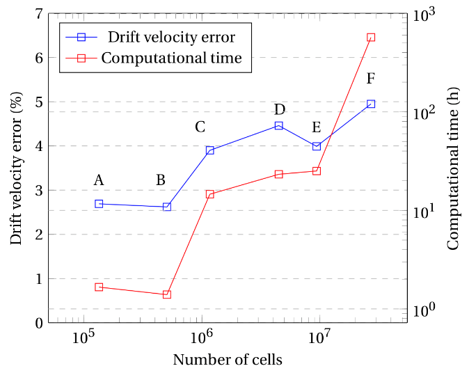
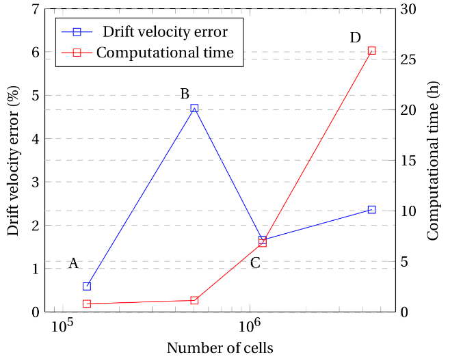
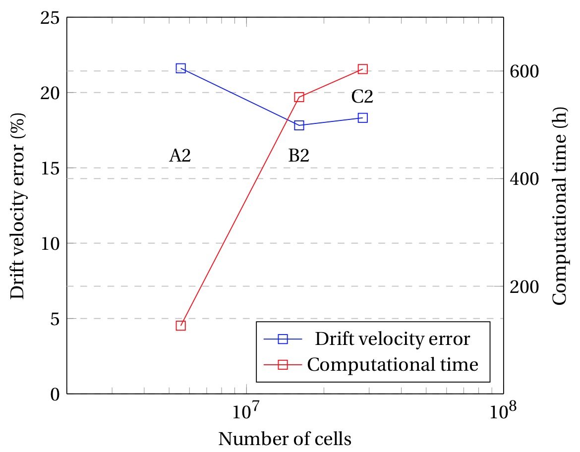
Figure 3. Mesh Independence results for Water on a (a) horizontal setting (b) 30º inclined setting (c) Generic high viscosity Oil. The simulations were performed with virtual machines with 8 cores and 32GB of Random-access (RAM) memory.
Table 3. Mesh Independence Tests established.
| Low-viscosity | High-viscosity | ||||||
| Fluid | Water | Mineral Oil | Generic Oil 1 | Generic Oil 2 | Generic Oil 3 | ||
| Case | Case 1 | Case 2 | Case 1 | Case 2 | - | - | - |
 |
1000 | 836 | 884 | 869 | 1410 | ||
 |
0.001 | 0.034 | 0.342 | 0.104 | 6.12 | ||
 |
0.072 | 0.03 | 0.029 | 0.029 | 0.087 | ||
| Pipe Diameter (m) | 0.0508 | 0.0508 | 0.044 | 0.044 | 0.0508 | 0.0508 | 0.0373 |
| Inclination Angle (°) | 0 | 30 | 0 | 30 | 0 | 10 | 0 |
| Distance travelled (m) | 0.5 | 0.5 | 0.5 | 0.5 | 0.5 | 0.5 | 0.25 |
| Source of comparison | [44] | [44] | This study | This study | [10] | [44] | [9] |
In the interest of comparing the CFD and the experimental data gathered on the present study, Fig. 4 (a) and Fig. 4 (b) were constructed by taking into account all the data available for all fluids and every different operational arrangement. In these figures, it can be appreciated that the great majority of the CFD data does not differ from its experimental counterpart by more than 10%. In fact, Fig. 4 (b) shows that only 15 out of 279 data points, which corresponds roughly to 5% of the data gathered, surpasses a drift velocity deviation of 10%. Moreover, most of the simulations carried out, corresponding to roughly 84% of the data gathered (235 out of 279 data points), predict a drift velocity with an experimental error below 5%.
From Fig. 4 (a) and Fig. 4 (b) it can also be noted that the highest drift velocity errors were observed for the lowest drift velocities, which translates into high viscosity fluids, as it was expected from the results obtained on the mesh independence test. The CFD model proposed predicts accurately the drift flux behavior for low viscosity fluids in any operational arrangement but struggles to simulate appropriately this phenomenon for fluids with higher viscosities. In general, the CFD model tends to overestimate the viscous effect on the drift velocity, predicting slower velocities than the experimental data observed. This observation will be analyzed in further detail in the upcoming sections. The overvalued viscous effect can be easily observed for the data point corresponding to -45% deviation. The minus sign refers to the fact that the CFD velocity is slower than the one determined experimentally. Additionally, the CFD model fails to estimate correctly the surface tension effect of the IsoparL, as it will be seen in Fig. 6, the drift velocity measured experimentally is much higher than the predicted in CFD.
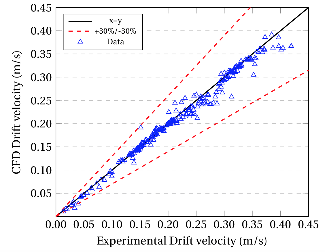
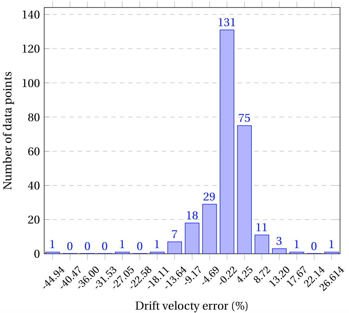
Figure 4. (a) CFD vs. Experimental drift velocity for all the operating conditions and fluids tested. (b) Distribution of the error.
3.2. Drift Flux Behavior Across the Pipe’s Length
From Fig. 5 (a) it can be appreciated that the drift velocity tends to decrease along the pipe´s length more prominently as the viscosity of the liquid phase increases. This can be explained through the predominant forces on each fluid, considering the Reynolds number relationship between inertial and viscous forces. The maximum Reynolds numbers for each of the cases considered on Fig. 5 are shown in Table 4 below:
Table 4. Maximum Reynolds numbers (CFD).
| Fluid | Re (D=44mm, |
Re (D=44mm, |
Re (D=17mm, |
Re (D=17mm, |
| Maple Syrup | - | 27.4105 | - | - |
| Hydraulic Oil | 108.261 | 136.729 | 5.260 | 23.682 |
| Olive Oil | 158.640 | 198.825 | 10.729 | 34.967 |
| Sunflower Oil | 185.627 | 230.636 | 13.485 | 41.524 |
| Mineral Oil | 337.074 | 419.237 | 33.110 | 76.709 |
| IsoparL Oil | 7453.711 | 8731.060 | 1442.634 | 1688.504 |
| Water | 13406.459 | 17457.640 | 2019.002 | 3259.187 |
For Reynolds over 7000, corresponding to water and IsoparL Oil in the 44 mm pipe, the inertial forces are predominant over the viscous forces. This implies that there will be no significant obstruction for the penetration of the gas bubble, maintaining the drift velocity constant. On the other hand, for low Reynolds number under 500, the viscous forces will be predominant over the inertial. Therefore, these forces will represent a significant energetic barrier for the gas bubble to overcome as it travels along the pipe, which will cause the bubble to slow down. In contrast, Fig 5 (b) shows predominant inertial forces over the viscous for all fluids in the inclined setting, keeping the drift velocity constant along the pipe length except for very viscous fluids, as seen for maple syrup. As mentioned in the previous section, the CFD model tends to overestimate the viscous effect on the drift velocity for high viscosity fluids, which causes a higher descent of the drift velocity along the pipe´s length compared to the experimental observations. This occurs due to the inclusion of the IMD model, as mentioned in section 2.2.2, given that it adds extra momentum dissipation in the proximity of the free surface [29]. This dissipation is defined by an interface artificial viscosity parameter which corrects the discontinuities in the solution fields, but adds an extra viscous term on the gas-liquid interface solution. Therefore, there will an additional viscous force which is not real and may affect the predicted motion of the bubble in CFD. A possible solution would be to study the high viscosity scenarios with different (or null) aritificial viscosities and evaluate the minimum required value to guarantee the dissipation of parasitic currents in the free surface without compromising the results. Additionally, a mesh quality test could be carried out in order to improve the possible discontinuities across the interface and guarantee less parasitic currents being generated due to discretization errors.
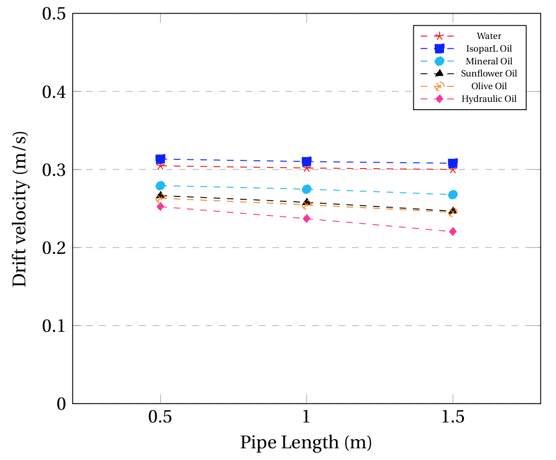
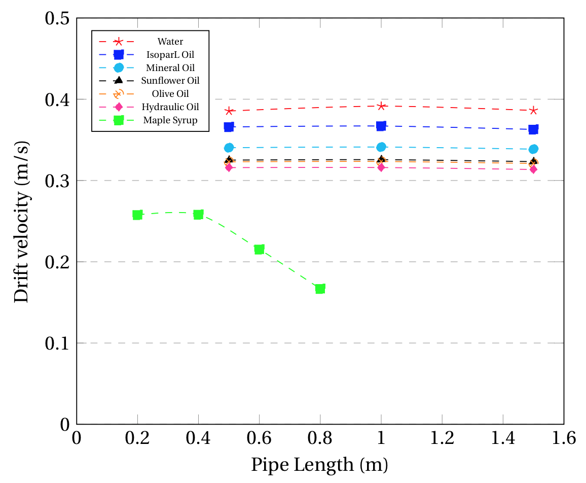
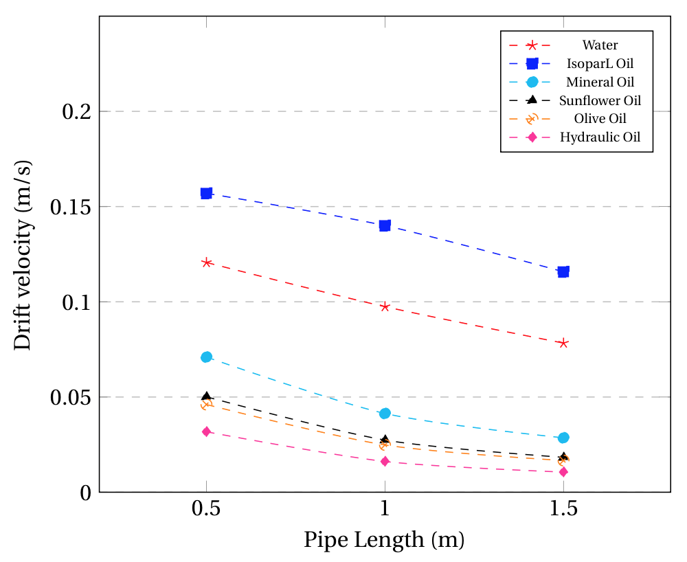
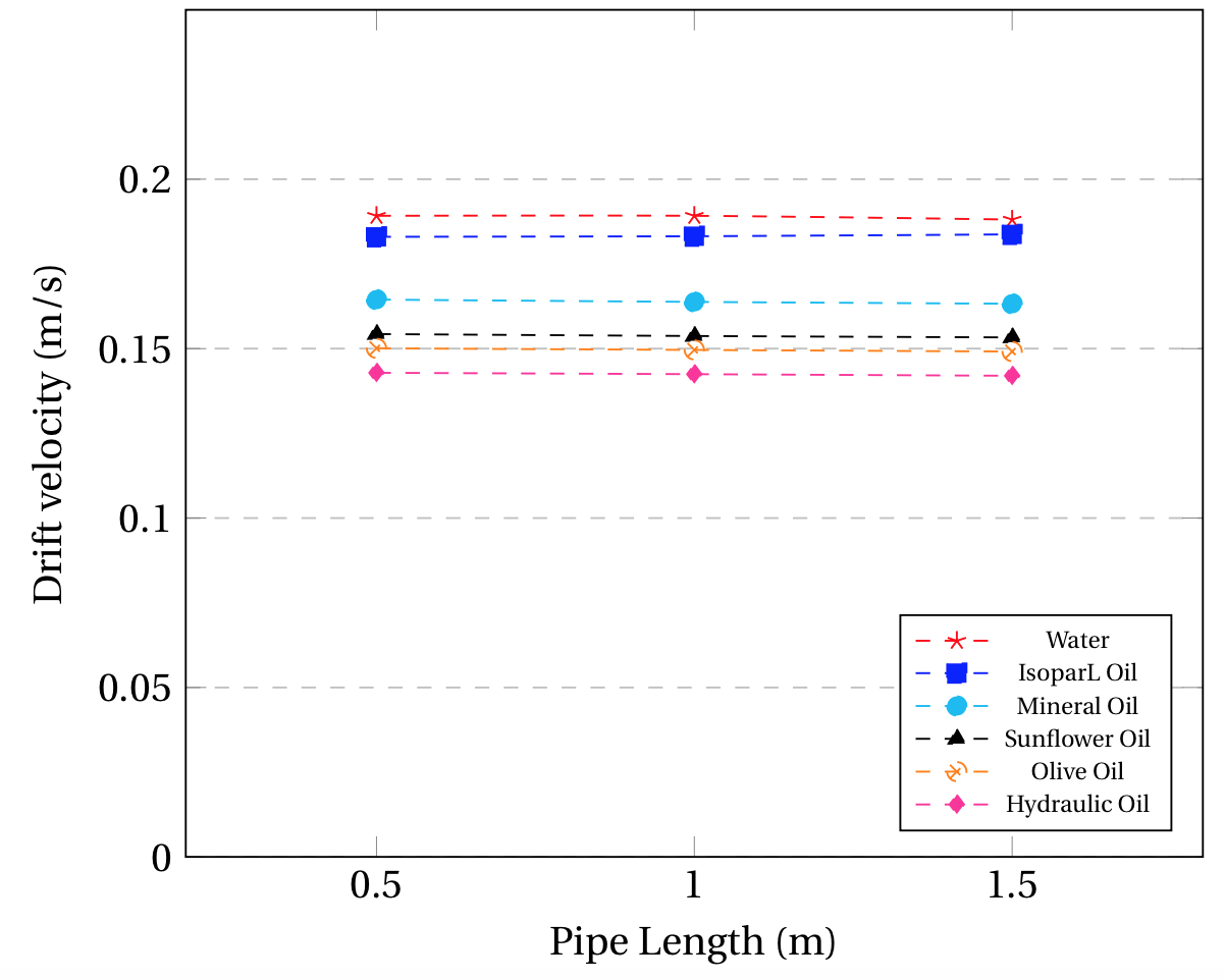
Figure 5. CFD results for the drift velocity behavior across the pipe length for Newtonian Fluids in (a) 44 mm and 0° (b) 44 mm and 40° (c) 17 mm and 0° (d) 17 mm and 40°.
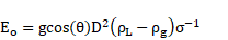
A similar case is observed for Fig. 5 (c) and (d) but between capillary/surface tension and gravitational forces described by the Eötvös number. By calculating the Eö number as reported in literature [1], it can be observed that all fluids in the 17 mm pipe have values under 100, which corresponds to dominant capillary forces over gravitational [14]. On the contrary, all fluids on the 44 mm pipe have Eö numbers over 100, regardless of the fluid considered. In Fig. 5 (c) it can be appreciated that the drift velocity decreases considerably along the pipe’s length for all fluids, regardless of their viscosity, opposite to the behavior observed for low viscosity fluids on the 44 mm pipe. This is due to the predominant capillary forces on the 17 mm pipe, which affect the penetration of the gas bubble on all fluids due to surface tension forces, slowing it down as it travels along the pipe. For the inclined configuration of the 17 mm pipe (Fig 5 (d)), it can be appreciated that the capillary forces are no longer significant on the system, as the drift velocity remains constant for all fluids, regardless of their viscosity and their Eö number. The reason for this observation may be considered from the Fr number comparison between the operational arrangement considered on Fig. 5 (c) and Fig. 5 (d). As seen on Eq (2), the Fr number depends on the type of fluid, the diameter of the pipe and the drift velocity. Given that Fig. 5 (c) and Fig. 5 (d) consider the same pipe and fluids, the only difference will be on the drift velocity, which is higher in all cases in Fig. 5(d). This means that the Fr number for the inclined configuration will be higher, which implies a higher contribution of inertial forces on the motion of the bubble. Therefore, inclined systems will have predominant inertial and gravitational forces.
3.3. Relationship Between the Drift Velocity and Inclination Angle
The results obtained through the CFD model shown in Fig 6 (b) are in good agreement with the experimental results obtained by Moreiras (2014) [1] and Gockal (2009)[44]. From Fig 6 (a) and (b) the drift velocity tends to reach a plateau as the angle increases up to 40º, regardless of the viscosity of the fluid. This plateau is caused by the fact that the inertial forces become predominant over the viscous or capillary forces for higher inclination angles, as seen in the previous section. Therefore, as the viscous forces are less representative on the motion of the gas bubble, the drift velocity value will tend to be constant and will depend entirely on the inertia associated with the gas bubble’s motion on each fluid. The only strong divergence to this pattern is the IsoparL Oil measured experimentally for the 40º setting, as it keeps increasing almost linearly with increasing angle. This implies that the CFD simulation does not model appropriately the effects of surface tension for this oil, as previously discussed in section 3.1.
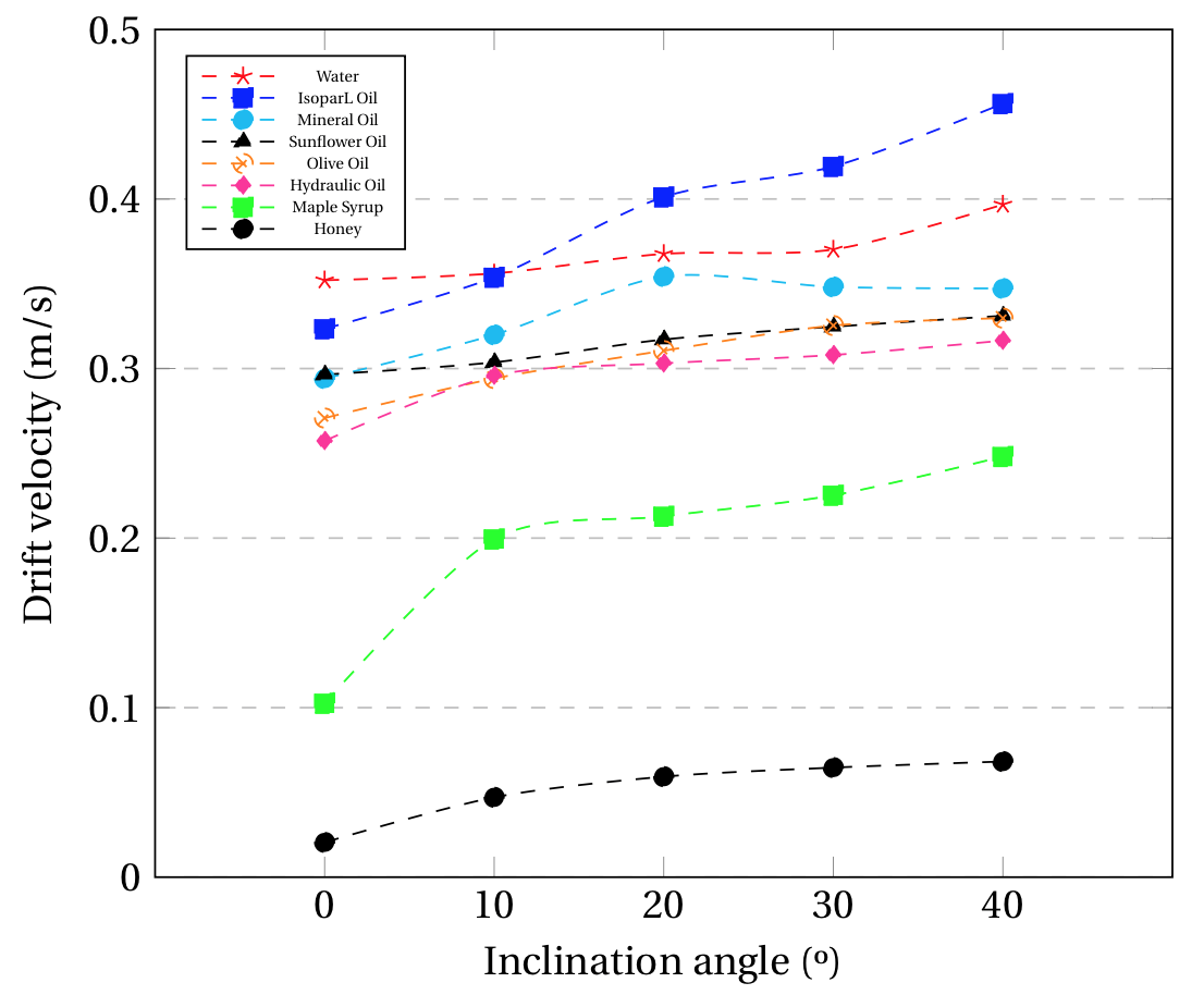
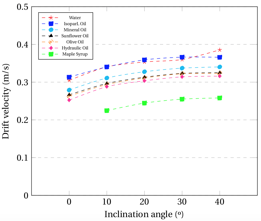
Figure 6. Drift velocity behavior against the angle of inclination for Newtonian Fluids in (a) Experimental (b) CFD, considering a 44 mm pipe and a measurement at 0.5 m along the pipe´s length.
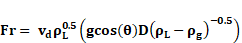
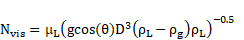
3.4. Froude Number vs Viscosity Number
The calculation for the Froude and viscosity number was done following the equations established by Moreiras (2014)[1]. An inverse exponential relationship was observed for all inclination angles between the Fr and Nvis calculated at a distance of 0.5 m along the pipe, which is in good agreement with the results reported by Moreiras (2014) [1]. From Fig. 7 (a) it can be noted that, in general, the Fr calculated with the experimental drift velocity measured is slightly larger than those predicted by the CFD model. This observation accounts for the over estimation of the viscous effect on the CFD model as commented on previous sections, which results in lower drift velocities than the observed. The decrease of the Fr against the Nvis becomes less prominent as the inclination angle increases, which translates into the dominant inertial forces observed for high inclination angles over viscous or capillary forces. Additionally, it can be noted that the rate at which the Fr decreases against the Nvis shows a similar pattern between inclined pipelines, especially for high viscosity fluids (high Nvis). However, this rate of decrease changes significantly from a horizontal pipeline to an inclined one, as can be seen in Fig. 7 (b,c). The inverse exponential relationship described between Fr and Nvis numbers is described through Eq (17).

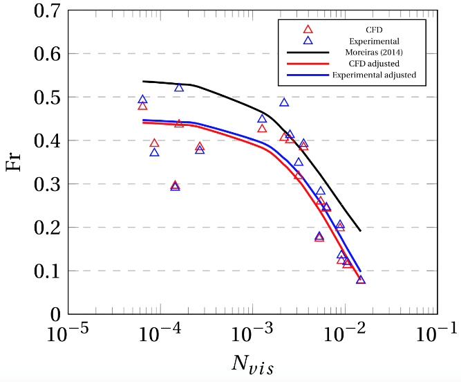
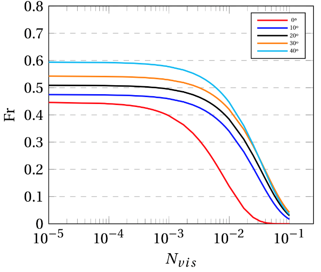
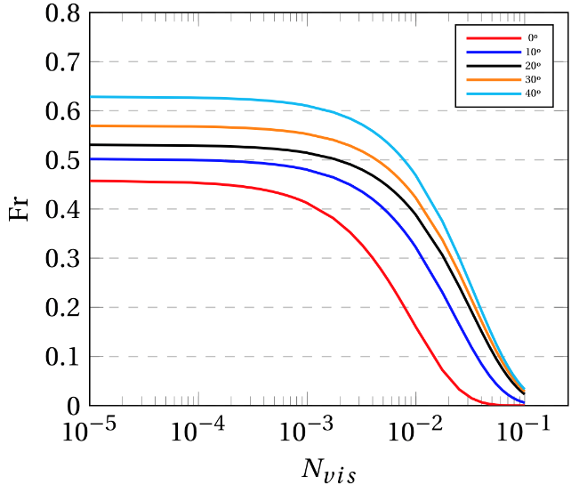
Figure 7. (a) Froude vs Viscosity number at 0° for Newtonian fluids, (b) Adjusted exponential function for Newtonian fluids (CFD) (c) Adjusted exponential function for Newtonian fluids (Experimental).
The fitting parameters for Eq (17) used to construct the adjusted experimental and CFD curves for all inclination angles as seen in Fig. 7 (b,c) are presented on Table 5.
Table 5. Adjusted parameters for Fr vs Nvis for each inclination angle.
| Inclination (º) | 0 | 10 | 20 | 30 | 40 |
| a (CFD) | 0.446 | 0.475 | 0.509 | 0.542 | 0.594 |
| b (CFD) | 117.7 | 33.51 | 28.27 | 25.62 | 28.60 |
| a (experimental) | 0.458 | 0.502 | 0.531 | 0.570 | 0.628 |
| b (experimental) | 105.4 | 44.46 | 31.37 | 29.90 | 29.46 |
From Fig. 8 it can be appreciated that Non-Newtonian fluids have smaller Fr numbers as compared to Newtonian fluids, given their high viscosity at low shear rates which occurs specially on a horizontal setting. Fig. 8 (a) and (b) shows a rapid decrease of the Fr for higher Nvis and smaller inclination angles. A drastic change in the Fr can be observed between the inclined pipelines and the horizontal setting, having smaller values by one order of magnitude. This behavior can be explained by the fact that, as opposed to inclined pipelines, the evacuation of the fluid on the horizontal case is caused only by the pressure difference between the initially sealed pipeline and the atmosphere, as there is no gravitational component influencing the motion of the gas bubble. Therefore, the shear rates occurring as the gas penetrates will be smaller to those on the inclined pipe, which implies that the effective viscosity of the liquid phase will be considerably larger. Consequently, the viscous forces that must be overcome are larger for the horizontal setting, resulting in smaller drift velocity values.
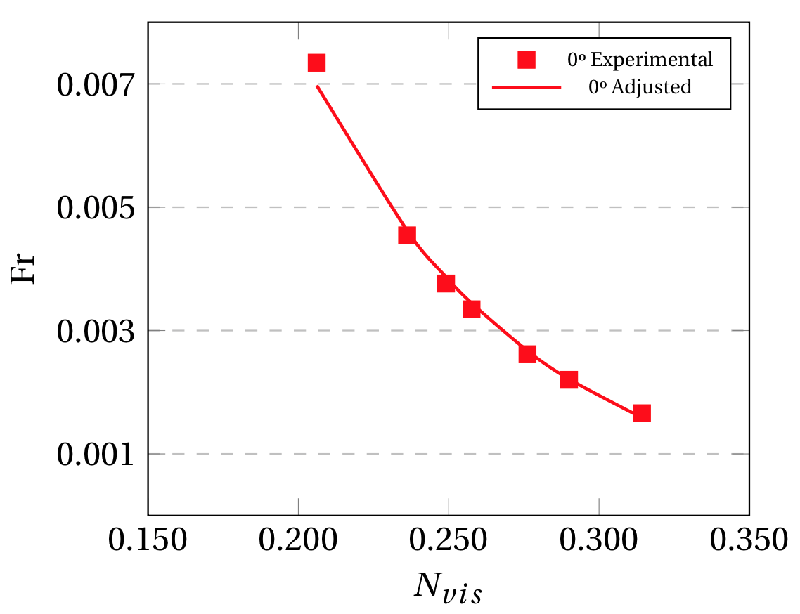
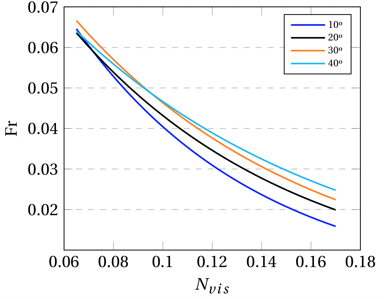
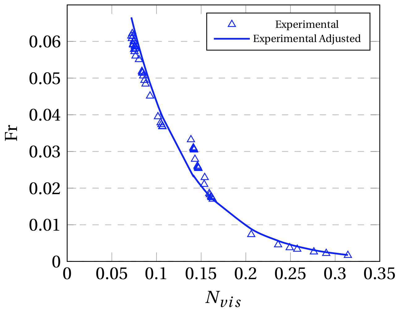
Figure 8. (a), (b) Adjusted experimental exponential functions and (c) Fr vs Nvis experimental data for Non-Newtonian fluids.
The fitting parameters used to construct the adjusted experimental curves for all inclination angles as seen in Fig. 8 (a,b) are presented on Table 6.
Table 6. Adjusted parameters for Fr vs Nvis for each inclination angle.
| Inclination (º) | 0 | 10 | 20 | 30 | 40 |
| a (experimental) | 0.117 | 0.154 | 0.131 | 0.130 | 0.115 |
| b (experimental) | 13.690 | 13.380 | 11.060 | 10.370 | 9.051 |
Fig. 8 (c) particularly was fitted to Eq (18) as shown further on. This figure shows the overall tendency between Fr and Nvis for all the experimental data gathered for Non-Newtonian fluids. It can be observed that this tendency may be interpreted as a continuation of the correlation suggested by Moreiras (2014) [1] for higher Nvis values, regardless of the operational settings considered. Even though it was observed that the rheological nature plays a fundamental role on the drift velocity measured, the Fr vs Nvis tendency observed for Newtonian fluids will still holds its relevancy for Non-Newtonian fluids with shear thinning characteristics.

4. Conclusions
The CFD and experimental modelling of the drift flux of a penetrating gas bubble into several fluids with different physical properties at varying pipe diameters, lengths and inclination angles was the focus of the present study. From the results obtained, it can be first concluded that the proposed CFD model can correctly estimate the drift velocity behavior for low viscosity fluids and calculates it adequately for high viscosity fluids, maintaining deviations under 10% for most of the cases studied. Only 15 data points out of 279 (roughly 5% of the data) have an error higher than 10% when compared with experimental data, and only 1 data point, corresponding to a high viscosity case, is above a 30% deviation as seen in Fig. 4. This data point represents an interesting case for further research given the satisfactory results obtained for the rest of the data points with the CFD model proposed.
The drift velocity across the pipe´s length tends to decrease for dominant capillary and viscous forces on Newtonian fluids, in which the condition of E <100 or Re<500 was fulfilled and a horizontal setting was considered. However, for dominant inertial and gravitational forces, the drift velocity maintained a constant value along the pipe’s length. For inclined configurations, it was found that, regardless the dominant forces, the drift velocity will always maintain a constant value. The behavior of the drift velocity against the angle of inclination showed a plateau region around 40º degrees of inclination for all fluids, despite of their viscosity. This behavior was in good correspondence with the data reported in literature [1]. This plateau region corresponds to the shift of dominant forces, in which the viscous/capillary forces become less significant on the penetration of the gas bubble and the inertia associated with its motion governs the phenomena. Therefore, the drift velocity will maintain constant values for inclination angles around this plateau region.
As for the behavior of the Froude number against the viscosity number, it can be concluded that, for both, Newtonian and Non-Newtonian fluids, the Froude number tends to decrease exponentially with an increase in the Viscosity number regardless of the operational conditions considered. This relationship is also in good agreement with results given in literature [1]. This decay becomes less prominent as the inclination angle increases. Therefore, it was found that the highest rate of change for the Froude number with the Viscosity number is observed at 0º for all fluids tested in this study. This behavior was attributed to the fact that, when the pipeline is positioned completely horizontally, only the pressure gradient between the pipe and the atmosphere produces the evacuation of the liquid and the entry of the bubble, whereas, in inclined pipelines, the gravitational acceleration has an additional contribution which affects the dominant forces of the system and the rheological behaviour of Non-Newtonian fluids. It was concluded that the rheological nature of the fluids has an important influence on the behaviour of the drift velocity observed.
Lastly, it can be stated that this research work provides insights into the behavior of the drift flux that could be applied to more viscous fluids that better resemble the properties of the ones found in the O&G industry. Moreover, the trends and relationships found in this study can be extrapolated to predict parameters of interest in heavy oil processing applications.
5. Future Work
As future work, the authors propose to develop a CFD model for Non-Newtonian fluids that considers the same cases tested on this study. A similar comparative and dimensionless analysis as the one carried out for Newtonian fluids is proposed as well. Additionally, authors propose to perform experimental and CFD tests on specific operational conditions related with the O&G industry in order to test the validity of the relationships found in this study.
References
[1] J. Moreiras, E. Pereyra, C. Sarica, and C. F. Torres, “Unified drift velocity closure relationship for large bubbles rising in stagnant viscous fluids in pipes,” Journal of Petroleum Science and Engineering, vol. 124, pp. 359–366, 2014. View Article
[2] R. D. Kaminsky, “Predicting single-phase and two-phase non-newtonian flow behavior in pipes,” Journal of Energy Resources Technology, vol. 120, no. 1, pp. 2–7, 1998. View Article
[3] G. A. Gregory and D. S. Scott, “Correlation of liquid slug velocity and frequency in horizontal cocurrent gas-liquid slug flow,” AIChE Journal, vol. 15, no. 6. pp. 933–935, 1969. View Article
[4] N. I. Heywood and J. F. Richardson, “Slug flow of air-water mixtures in a horizontal pipe: Determination of liquid holdup by γ-ray absorption,” Chemical Engineering Science, vol. 34, no. 1, pp. 17–30, 1979. View Article
[5] A. E. Dukler and M. G. Hubbard, “A Model for Gas-Liquid Slug Flow in Horizontal and Near Horizontal Tubes,”Industrial & Engineering Chemistry Fundamentals , vol. 14, no. 4, pp. 337–347, 1975. View Article
[6] T. B. Benjamin, “Gravity currents and related phenomena.,” Journal of Fluid Mechanics, vol. 31, no. 2, pp. 209–248, 1968. View Article
[7] M. E. Weber, “Drift in intermittent two phase flow in horizontal pipes,” The Canadian Journal of Chemical Engineering, vol. 59, no. 3. pp. 398–399, 1981. View Article
[8] K. Bendiksen, “An Experimental Investigation of the Motion of Long Bubbles in Inclined Tubes,” International Journal of Multiphase Flow, vol. 10, no. 4, pp. 467–483, 1984. View Article
[9] M. E. Weber, A. Alarie, and M. E. Ryan, “Velocities of extended bubbles in inclined tubes,” Chemical Engineering Science, vol. 41, no. 9, pp. 2235–2240, 1986. View Article
[10] B. Gockal, Q. Wang, H.-Q. Zhang, and C. Sarica, “Effects of High Oil Viscosity on Oil/Gas Flow Behavior in Horizontal Pipes,”, SPE Projects, Facilities & Construction, Society of Petroleum Engineers, pp. 1–11, 2008.
[11] G. Losi and P. Poesio, “An experimental investigation on the effect of viscosity on bubbles moving in horizontal and slightly inclined pipes,” Experimental Thermal and Fluid Science, vol. 75, pp. 77–88, 2016. View Article
[12] P. Andreussi, M. Bonizzi, and A. Vignali, “Motion of elongated gas bubbles over a horizontal liquid layer,” 14th International Conference on Multiphase Production Technology, France, pp. 309–318, 2009.
[13] L. F. Barceló, P. A. Caron, A. E. Larreteguy, R. Gayoso, F. Gayoso, and G. Guido Lavalle, “Análisis del comportamiento de equipos separadores de agua-petróleo usando volumenes finitos y el modelo del drift flux,” Computational Mechanics, vol. XXIX, no. 87, pp. 8463–8480, 2010.
[14] M. Ramdin and R. Henkes, “Computational Fluid Dynamics Modeling of Benjamin and Taylor Bubbles in Two-Phase Flow in Pipes,” Journal of Fluids Engineering, vol. 134, no. 4, p. 041303, 2012. View Article
[15] R. F. Kroes and R. A. W. M. Henkes, “CFD for the motion of elongated gas bubbles in viscous liquid,” BHR Gr. - 9th North American Conference on Multiphase Technology, Canada, no. 1, pp. 283–298, 2014.
[16] M. Lu, “Experimental and computational study of two-phase slug flow,” Imperial College of London, 2015.
[17] B. Sanderse, M. Haspels, and R. A. W. M. Henkes, “Simulation of Elongated Bubbles in a Channel Using the Two-Fluid Model,” Journal of Dispersion Science and Technology, vol. 36, no. 10, pp. 1407–1418, 2015. View Article
[18] A. A. Bishop and S. D. Deshande, “Non-newtonian liquid-air stratified flow through horizontal tubes-ii,” International Journal of Multiphase Flow, vol. 12, no. 6, pp. 977–996, 1986. View Article
[19] I. Iliuta, F. C. Thyrion, and O. Muntean, “Hydrodynamic characteristics of two-phase flow through fixed beds: Air/newtonian and non-newtonian liquids,” Chemical Engineering Science, vol. 51, no. 22, pp. 4987–4995, 1996. View Article
[20] M. Dziubinski, H. Fidos, and M. Sosno, “The flow pattern map of a two-phase non-Newtonian liquid-gas flow in the vertical pipe,” International Journal of Multiphase Flow, vol. 30, no. 6, pp. 551–563, 2004. View Article
[21] D. J. Nicklin, M. A. Wilkes, and J. F. Davidson, “Two-Phase Flow in Vertical Tubes,” Transactions of the Institution of Chemical Engineers, vol. 40, pp. 61–67, 1962.
[22] G. B. Wallis, One-dimensional two-phase flow. New York, McGraw-Hill, 1969.
[23] Y. Taitel and D. Barnea, Encyclopedia of Two Phase Heat Transfer and Flow I. World Scientific Publishing Co., 2015.
[24] M. Ishii and T. Hibiki, Thermo-fluid dynamics of two-phase flow. 2006.
[25] L. Cheng, Frontiers and Progress in Multiphase Flow I. Springer, 2014.
[26] B. Jeyachandra, “Effect of Pipe Inclination on Flow Characteristics of High Viscosity Oil-Gas Two-Phase Flow,” The University of Tulsa, 2011.
[27] C. T. Crowe, Multiphase Flow Handbook, vol. 1218, no. 36, 2006.
[28] R. Darby, Chemical Engineering Fluid Mechanics, Revised and Expanded, vol. 2. New York, Taylor & Francis, 2001.
[29] Siemens, “STAR CCM+ Documentation.” Siemens, NY, 2016.
[30] M. Peric, “Polyhedral Grids In STAR-CCM +.” CD-ADAPCO, pp. 1–31, 2017.
[31] R. B. Bird, W. E. Stewart, and E. N. Lightfoot, “Transport Phenomena,” J. Wiley, 2007.
[32] C. W. Hirt and B. D. Nichols, “Volume of fluid (VOF) method for the dynamics of free boundaries,” Journal of Computational Physics, vol. 39, no. 1, pp. 201–225, 1981.
[33] H. Pineda, T.-W. Kim, N. Ratkovich, and E. Pereyra, “CFD Modelling of High Viscosity Liquid-Gas Two-Phase Slug Flow,” Universidad de los Andes, 2016.
[34] C.-M. Lee and T. Frankiewicz, “The Design of Large Diameter Skim Tanks Using Computational Fluid Dynamics (CFD) For Maximum Oil Removal,” in 15th Annual Produced Water Seminar, 2005.
[35] H. Yang, J. Lu, and S. Yan, “Preliminary Numerical Study on Oil Spilling from a DHT,” Twenty-fourth International Ocean and Polar Engineering Conference, vol. 3, no. 1994, pp. 610–617, 2014.
[36] J. Monroy and M. Sato, “A VOF Numerical Model of Storm Waves on Coral Reefs,” in Proceedings of the Thirteenth International Offshore and Polar Engineering Conference, pp. 721–728, 2003.
[37] S. Jeon, S. Kim, and G. Park, “CFD simulation of condensing vapor bubble using VOF model,” International Journal of Physical and Mathematical Sciences, World Academy of Science, Engineering and Technology, vol. 3, no. 12, pp. 209–215, 2009.
[38] S. Lo and A. Tomasello, “Recent progress in CFD modelling of multiphase flow in horizontal and near-horizontal pipes,” 7th North American Conference on Multiphase Technology, BHR Group, pp. 209–219, 2010.
[39] D. J. E. Harvie, M. R. Davidson, and M. Rudman, “An analysis of parasitic current generation in Volume of Fluid simulations,” Applied Mathematical Modelling, vol. 30, no. 10, pp. 1056–1066, 2006. View Article
[40] V. Hernandez-Perez, M. Abdulkadir, and B. Azzopardi, “Grid Generation Issues in the CFD Modelling of Two-Phase Flow in a Pipe,” The Journal of Computational Multiphase Flows, vol. 3, no. 1, pp. 13–26, 2011. View Article
[41] F. White, “Fluid Mechanics,” McGraw-Hill, New York, p. 862, 2010.
[42] H. Schlichting, Boundary layer theory. 2017.
[43] Ansys, “Ansys fluent 12.0 Theory Guide,” 2009.
[44] B. Gokcal, A. S. Al-Sarkhi, and C. Sarica, “Effects of High Oil Viscosity on Drift Velocity for Horizontal and Upward Inclined Pipes,” SPE Projects, Facilities & Construction, vol. 4, no. 02, pp. 32–40, 2009. View Article