Journal of Fluid Flow, Heat and Mass Transfer (JFFHMT)

ISSN: 2368-6111

1. Introduction

Twist-drill machining is a process of creating cylindrical holes frequently used in the manufacture of cars, trains, planes and ships and are typically comprised of two components, the drill and the cutting tool (referred to as the drill bit) [1]. The drill rotates and supplies forces to the drill bit, while the drill bit applies the forces to cut the workpiece. The improvement of drill bit performance is of particular interest to the manufacturing industry in order to reduce component costs and improve component quality. However, one of the central challenges of increasing productivity is the management of large thermo-mechanical loads.

 

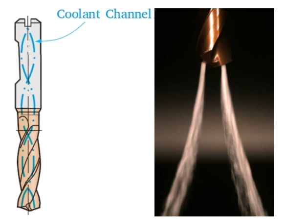
Since the first report of cutting fluids in 1894 by F. Taylor, liquid coolants have been increasingly used to handle these loads and extend tool life [1]. One common method of coolant application is via through-tool internal coolant channels, illustrated in Figure 1, to supply liquid emulsion coolant directly to the point geometry to transport thermal energy away from the tool [2] and aid chip evacuation [3]. The experimental observation of coolant application is particularly challenging due to the combination of small enclosed borehole geometry and large tool angular velocities. As a result, it is difficult to improve the usage of coolant with little knowledge of the underlying delivery mechanisms. In light of these limitations, studies are typically limited to post-experiment tool inspection [5, 6] or through cutting force telemetry data analysis. These experimental challenges have led to numerous research papers adopting Computational Fluid Dynamics (CFD) to numerically study coolant performance.

CFD has been employed to investigate a number of different drilling applications such as internal coolant channels in oil-well drilling [7], tool wear in the oil and gas industry [8] and MQL applications [3]. In twist-drill machining, research by Obikawa et al. [9] studied coolant flow between the tool flank face and the workpiece surface in response to changes in flow rate. This work found that the narrow space between the flank face and workpiece limited the supply of coolant and an increase in flow rate improved supply of coolant to the cutting geometry. Beer et al. [6] used a CFD model, validated by tool wear inspections, to investigate the effects of grooves in the flank face on tool life and hole quality in the drilling of Inconel 718. The addition of grooves in the flank face was found to increase tool life by up to 50%. A recent study by Fallenstein et al. [10] used CFD to study the single phase flow of coolant within the borehole and predict the amount of heat removed by coolant. Both channel positioning and flow rate were found to have a significant impact on the amount of heat removed from the tool. The benefit of increased flow rate was consistent across all designs and channel circumferential position had a greater effect on heat transfer than the radial positioning.  Özkaya et al. [5] also employed a single-phase model to study the effects of coolant hole position and flow rate on tool-coolant heat transfer in Inconel 718 drilling. It was found that coolant is primarily distributed into the flute and identified ‘dead’ zones by the cutting edge corner. Increasing the supply pressure was found to have the greatest impact on tool cooling as well as increasing the coolant supply to these stagnant zones.

This work contributes to the existing literature on coolant flow as it is the first to use multi-phase modelling methods to study coolant distribution regions which have not previously been documented. Issues with swept meshing approaches are addressed using a Finite Element (FE)-based model to simulate the machining process and calculate the borehole geometry profile and chip formation. The distribution of coolant between the tool, borehole and chip is modelled using a Finite Volume (FV)-based numerical method which uses the Volume Of Fluid (VOF) method to track the delivery of coolant. This numerical approach has been combined with response surface models to analyse channel positioning effects on domain filling behaviour and the percentage lubricated area of the tool. Finally, visual analysis of numerical tool surface coolant distributions is used to study tool component wetting in response to changes in channel positioning.

2. Model Formulation

The numerical model outlined in this article is constructed from two loosely coupled numerical models.

The first model, which will be referred to as the machining model, is a FE-based model of the machining process which is responsible for calculating the formation of the workpiece and chip. These simulations are carried out using ThirdWave Systems AdvantEdge. Further information regarding simulation set up is provided in Section 2.1.

The second model, referred to as the fluid model, is a FV-based model implemented in OpenFOAM [11] and uses the workpiece geometry calculated in the machining model to create a computational mesh accounting for the tool, chip and work-piece geometry. The fluid model is a two-phase flow model which uses the VOF method to track the coolant/air interface for realistic tool-chip geometries. Further details are given in Section 2.2.

2. 1. Machining Model

This work uses ThirdWave Systems AdvantEdge version 7.1 simulation package to calculate the workpiece formation. The software, presented originally in [12], is used to simulate solid carbide drilling of steel. The software is based on a dynamic explicit Lagrangian FE model which employs adaptive remeshing to minimise element distortion. The tool used for this model is an 8mm diameter Sandvik Coromant CoroDrill 460 made from carbide grade H10F and the workpiece material is AISI-4140. The material model used for the workpiece and tool are part of the standard material library included in the software. The simulation used the default friction and heat transfer models and parameters; workpiece starting depth of 8mm with initial temperature of 20 degrees Celsius was used. The simulation calculated 3 complete tool rotations to ensure a large continuous chip had formed using a spindle speed of 3970 RPM and 0.2mm feed per revolution. Dynamic mesh refinement is used locally around the tool cutting edge to ensure adequate mesh resolution to resolve the cutting process; note that no mesh coarsening was authorised in order to ensure that it always provides an accurate representation of the complete tool and chip geometry. In order to ensure an accurate representation of edge rounding a minimum element edge length of 0.002mm was used. The initial workpiece mesh consists of 138,053 tetrahedral elements, and the number of elements increases as the cutting progresses due to the adaptive remeshing. A total of 2139117 time steps were needed to complete the simulation as well as 1369 mesh refinement steps. Eight Central Processing Units (CPU) were used to carry out the simulation on two Intel Zeon E52630 processors with a total CPU time of 292h 32min.

2. 2. Fluid Model

The present work considers water-miscible coolant which is approximately 95% water, the remaining portion consists of an oil with similar properties to water and therefore coolant is modelled as water. Both the air and coolant phases are treated as Newtonian and incompressible. A similar approach to the VOF method described in [13] is used to track the large quantities of coolant [14], as implemented in the OpenFOAM CFD library [11]. The formulation of the model is given below:

Where   is velocity and is the relative velocity defined as , where subscript l and g correspond to the liquid coolant and gas phases respectively. is the volume fraction and  is the volume averaged viscosity defined as:

where and  .   is the volume averaged density given by:

with   and . In order to simplify the definition of boundary conditions pressure is modified so that a single pressure system is considered, this is necessary due to the normal component of the pressure gradient at stationary non-vertical no-slip walls being different for each phase. Here pressure is modified by the density gradient and the body force due to gravity given by . Where x is the position vector and acceleration due to gravity [15].

Surface tension is accounted for within the momentum equation by including it as a body force, . Surface tension at the liquid gas interface generates an additional pressure gradient, which is evaluated per unit volume using the continuum surface model formulation of Brackbill et al. [16]:

where is the surface tension,  is the normal vector of the interface, is the interface delta function and is the mean curvature of the interface defined as:

The presented VOF formulation has been evaluated against a range of multiphase flow problems, such as modulated jets [17], droplet impact and crater formation [18], film falling over turbulence wires [19] and inertia dominated and surface tension dominated flow regimes [15].

By weighing coolant captured in a container across a fixed time period the average fluid velocity exiting the tool was calculated at 80ms^-1. From this, the Reynolds number was calculated at approximately 79000 indicating that the flow is highly turbulent and is accounted for using the realisable turbulence model. The boundary conditions used specify the velocity at the inlet as 80ms^-1 and pressure zero gradient, at the outlet atmospheric pressure is specified and an outlet condition is selected for velocity. For the tool and workpiece walls zero velocity no slip conditions are specified and for pressure zero gradient. Standard  wall functions have been used as detailed in [20]. The effects of rotation were not included in this simulation as the inertia of the liquid phase dominates the Coriolis forces, following the findings of [21].

2. 3. Computational Geometry

The computational mesh for the fluid domain, the cavity inside the borehole surrounding the workpiece walls, chip and tool, is created with snappyHexMesh using the tool CAD geometry and the workpiece geometry calculated by the machining model as inputs.

The meshing process was initialised using a uniform grid of 778410 control volumes, and surface based refinement was then used to provide an additional level of refinement close to surfaces and corners.  The resulting mesh of the fluid domain includes the chip, the shape of the borehole bottom and the clearance between the tool margin and the workpiece wall. As a result of modelling the margin/workpiece clearance, there is no physical boundary preventing coolant recirculation between flutes. Therefore the fluid domain models both tool flutes, cutting edges and coolant channels. The resulting meshes were constructed from roughly 2 million control volumes with an average  of 24. Grid sensitivity was checked by comparing the results against another with 5 million control volumes and this was found to be sufficient as the discrepancy between the results was 1%.

3. Results

3. 1. Experimental Validation

The numerical model is validated experimentally using a sacrificial polymer coating to indicate coolant delivery regions. This analysis was performed by first coating the tool in a proprietary polymer made from Nitrocellulose and coloured to aid visual inspection, then inserting the tool into a pre-drilled blind hole of depth three times tool diameter 0.4mm from the borehole bottom. Coolant is supplied for 20 seconds before removing the tool and visually inspecting for surface regions where the polymer coating has been removed. The surface regions where the polymer coating has been removed indicates where coolant is supplied after exiting the tool. Experimental

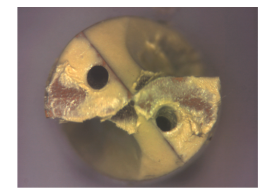
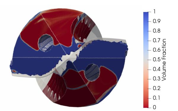
measurements are presented in Figure 3 and show that the polymer coating has largely been removed on the flank face between the coolant channel and the cutting edge and across the axial rake. Figure 4 shows the distribution of coolant predicted across the tool surface using CFD where the blue areas indicate zones supplied with coolant and the red areas indicate regions which are not supplied with coolant. The profile of coolant calculated by the CFD model is clearly in qualitative agreement with the profile shown in the experiment. Furthermore, the CFD model is also predicting that coolant is not directly supplied to the tertiary clearance or the tool flute, which is also reflected in the experimental results. An approximate quantitative comparison of the percentage of the tool primary and secondary clearance supplied with coolant is estimated by computational image analysis which showed that 55% of the polymer coating is removed in the experiments compared with 67% from the computations. More sophisticated methods of comparison will be developed in future work.

3. 2. Coolant Channel Analysis

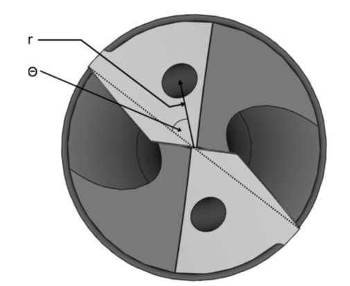
In this paper, the effects of coolant channel exit position on domain filling and tool wetting behaviour will be studied. Each coolant channel is specified relative to its radial positioning, and circumferential position, ,illustrated in Figure 5. In the following sections, each design has been analysed for its domain flooding behaviour and its tool wetting response. Domain flooding analysis calculates the percentage of the borehole flooded by coolant, or how long it takes for the cutting zone to become fully flooded. Both will influence drill cooling and are calculated by:

where  is the number of control volumes,  is the volume of control volume  and is the volume fraction calculated at control volume . To aid analysis this is represented as a percentage of the total domain volume.

Tool wetting calculates the area of the tool coated in coolant. This is calculated by:

where  is the number of faces used to represent the tool surface,  is the area of face  and  is the volume fraction of face . Tool wetting is represented in the later sections as a percentage of the total surface area.

3. 3. Response Surface Modelling

The effect of coolant channel exit circumferential positioning, , and radial positioning, , on tool wetting and borehole flooding is shown through response surfaces. To ensure a uniform distribution of numerical evaluations throughout the design space a Design of Experiments (DoE) was obtained using an Optimum Latin Hypercube sampling method consisting of 20 points in the domain  and , see e.g. [22]. Response surfaces are then constructed using a Moving Least Squares (MLS) metamodel from steady state CFD solutions of the samples. The DoE points and the calculated flooding and tool wetting responses are given in Table 1. The MLS metamodel uses a Gaussian weight decay function to determine the weighting of points in the regression analysis at each design point :

where  is the Euclidean distance between the design point  at which the MLS metamodel is being evaluated, and the ith DoE point , and  is the closeness of fit parameter. A large value of  ensures the MLS metamodel reproduces the known DoE point values accurately, whereas a smaller value of  can reduce the effect of numerical noise on the metamodel [23]. The values of  for the metamodel are selected by minimising the Root Mean Square Error (RMSE) between the predictions from the metamodel and those from the CFD at the DoE points. Following [24] Leave One Out (LOO) cross validation is used, where a DoE point is removed from the metamodel and a metamodel is created using the remaining 19 points. The removed point is used to evaluate the model RMSE. This is then repeated for every DoE point and the average RMSE across the set of 20 DoE points is calculated.

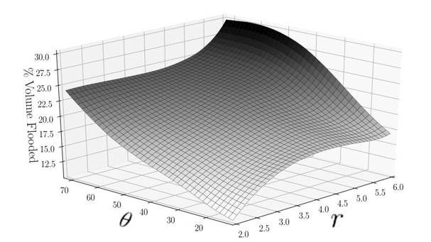
The response surface calculated for domain flooding is given in Figure 6 with an optimum  and RMSE of 0.9. Firstly the resulting surface shows that no designs fully flood the domain. The designs which fill the borehole cavity the most at approximately 30% have large circumferential and radial spacing. However, the designs which fill the fluid domain the least have the smallest radial distance and are positioned closer to the cutting edge. Finally, it was found using the response surface that borehole filling is most sensitive to  at smaller values of .

Table 1. Design of Experiments and CFD results.

Design#			% Flooded	% Wetted
1	2	27.71	13	38
2	2.21	65.6	22	48
3	2.42	52.97	19	44
4	2.63	37.18	17	40
5	2.84	18.24	15	35
6	3.05	62.45	22	48
7	3.26	49.81	20	43
8	3.47	30.87	18	38
9	3.68	15.08	17	43
10	3.89	71.92	24	51
11	4.11	40.34	21	44
12	4.32	59.29	23	50
13	4.53	24.55	19	43
14	4.74	46.66	23	53
15	4.95	11.92	17	40
16	5.16	68.76	25	51
17	5.37	34.025	21	42
18	5.58	56.13	26	55
19	5.79	21.39	19	39
20	6	43.5	28	53

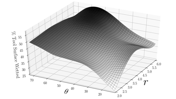
A metamodel showing the percentage of the tool surface coated in coolant as a function of r and  is given in Figure 7. The MLS surface was created using  and a resulting RMSE of 0.03. The results show that no design lubricates the entire tool and that there are regions of the surface geometry that are not supplied with coolant.

The design with global maximum surface wetting of 56% was found using a particle swarm genetic algorithm, which is located at  and . This combined with the flooding response surface show that designs with large and  flood the borehole the most and lubricate the greatest area of the tool.

3. 4. Wetting Profiles

The previously discussed metamodels are effective at giving an overview of the effects of radial and circumferential positioning of coolant channels. However, measuring the response of the system in terms of a percentage of the tool covered does not indicate which components of the external geometry are supplied with coolant. Figure 8 qualitatively analyses the distribution of coolant about the tool surface by colouring the tool geometry of each DoE point by the steady state distribution of coolant. In order to aid the visualisation the workpiece and chip have been subtracted from the image. Each design evaluated in Table 1 is given in Figure 8 and annotated

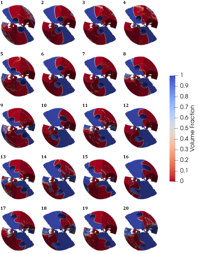
by its corresponding design number. In this figure, the tool surfaces are coloured by the volume fraction, where the blue areas indicate wetted areas () and red areas indicate areas of the surface which are not (). It can clearly be seen that all designs follow similar profiles; coolant is supplied directly to the flank face, the back of the cutting edge, across the axial rake and into the workpiece walls. However, the size of the flank face area supplied with coolant is shown to be sensitive to the location of the coolant channel exit position. From this collection of results, it can be seen that only a small amount of coolant is directed up the flute of the tool, which would otherwise be evidenced by more coolant up the secondary clearance or on the flute face. The amount of coolant directed across the axial rake appears to be influenced by the radial distance of the coolant channel more significantly than the circumferential positioning as designs with larger radial positioning are shown to provide more coolant to the axial rake of the tool than designs with smaller r. This suggests that tool designs which favour chip evacuation using coolant may benefit from positioning channels with large circumferential and radial positioning in order to increase flow to the axial rake, whereas tools which require increased heat transfer would benefit from minimising circumferential position to concentrate the delivery about the cutting edge. 

4. Conclusions

Previous research has shown coolant improves drill bit performance by lubricating the cutting zone, removing heat and aiding chip evacuation. The central motivation of this work is to understand how these improvements are achieved through studying how coolant is distributed inside the borehole. Previous CFD modelling of twist-drill coolant employed single phase formulations to predict trajectory and heat transfer. This work is the first to employ a multiphase CFD model to study the distribution and wetting profile in twist-drill machining. This is combined with a machining model to calculate a realistic borehole geometry for the CFD meshing process.

Response surface modelling of domain flooding shows that the position of the coolant channel does not significantly affect the cavity filling and no design fully floods the domain. The designs which maximise the domain flooding achieve approximately 30% flooding and maximise both circumferential and radial spacing. Wetting response surfaces found that no designs fully lubricated the tool, but tools with greater circumferential positioning cover a greater percentage area of the tool than channels with smaller circumferential positioning. Coolant channels which are located further from the centre of the tool also increased the percentage area of the tool coated in coolant, however the effects were less significant than circumferential positioning.

Profile wetting analysis was used to evaluate tool surface coolant distribution for each channel configuration to identify the geometry components which are supplied with coolant. All of the tested designs displayed a similar coolant distribution pattern where coolant is supplied along the tool flank face between the coolant holes and the cutting edge before being directed into the workpiece walls or across the tool axial rake. The results show that as the circumferential distance increases, a larger area of the flank face is coated in coolant. Small circumferential positioned coolant channels, which are closer to the cutting edge, appear to coat less of the tool with coolant but highly localise the wetting about the cutting edge. Finally, visual analysis of the CFD results showed that the quantity of coolant directed either to the tool margin or across the axial rake can be controlled through coolant channel positioning, channels with large  and  direct more coolant across the axial rake, while tools with small  direct less coolant across the axial rake.

Acknowledgements

The funding from Innovate UK in the form of Knowledge Transfer Partnership grant 009868 is gratefully acknowledged.

References

[1] R. Avila and A. Abrao, “The effect of cutting fluids on the machining of hardened AISI 4340 steel,” Journal of Materials Processing Technology, vol. 119, no. 1, pp. 21-26, 2001. View Article
[2] D. Haan, S. Batzer, W. Olson, and J. Sutherland, “An experimental study of cutting fluid effects in drilling,” Journal of Materials Processing Technology, vol. 71, no. 2, pp. 305-313, 1997. View Article
[3] D. U. Braga, A. E. Diniz, G. Miranda, and N. Coppini, “Using a minimum quantity of lubricant (mql) and a diamond coated tool in the drilling of aluminum–silicon alloys,” Journal of Materials Processing Technology, vol. 122, no. 1, pp. 127-138, 2002. View Article
[4] P. Zhang, N. Churi, Z. J. Pei, and C. Treadwell, “Mechanical drilling processes for titanium alloys: a literature review,” Machining Science and Technology, vol. 12, no. 4, pp. 417-444, 2008. View Article
[5] E. Özkaya, N. Beer, and D. Biermann, “Experimental studies and cfd simulation of the internal cooling conditions when drilling inconel 718,” International Journal of Machine Tools and Manufacture, vol. 108, pp. 52-65, 2016. View Article
[6] N. Beer, E. Özkaya, and D. Biermann, “Drilling of inconel 718 with geometry-modified twist drills,” Procedia CIRP, vol. 24, pp. 49-55, 2014. View Article
[7] F. A. R. Pereira, M. A. S. Barrozo, and C. H. Ataíde, “Cfd predictions of drilling fluid velocity and pressure profiles in laminar helical flow,” Brazilian Journal of Chemical Engineering, vol. 24, pp. 587- 595, 12, 2007.
[8] G. Watson, N. Barton, G. Hargrave et al., “Using new computational fluid dynamics techniques to improve pdc bit performance,” SPE/IADC Drilling Conference. Society of Petroleum Engineers, 1997. View Article
[9] T. Obikawa and M. Yamaguchi, “Computational fluid dynamic analysis of coolant flow in turning,” Procedia CIRP, vol. 8, pp.271-275, 2013. View Article
[10] F. Fallenstein and J. Aurich, “Cfd based investigation on internal cooling of twist drills,” Procedia CIRP, vol. 14, no. 0, pp. 293-298, 2014, 6th CIRP International Conference on High Performance Cutting, HPC2014. View Article
[11] H. G. Weller, G. Tabor, H. Jasak, and C. Fureby, “A tensorial approach to computational continuum mechanics using object-oriented techniques,” Computers in Physics, vol. 12, no. 6, pp. 620-631, 1998. View Article
[12] T. Marusich and M. Ortiz, “Modelling and simulation of high-speed machining,” International Journal for Numerical Methods in Engineering, vol. 38, no. 21, pp. 3675-3694, 1995.
[13] C. W. Hirt and B. D. Nichols, “Volume of fluid (vof) method for the dynamics of free boundaries,” Journal of computational physics, vol. 39, no. 1, pp. 201-225, 1981. View Article
[14] O. Ubbink, “Numerical prediction of two fluid systems with sharp interfaces,” Ph.D. Dissertation, University of London UK, 1997.
[15] S. S. Deshpande, L. Anumolu, and M. F. Trujillo, “Evaluating the performance of the two-phase flow solver interfoam,” Computational Science & Discovery, vol. 5, no. 1, p. 014016, 2012. View Article
[16] J. Brackbill, D. B. Kothe, and C. Zemach, “A continuum method for modeling surface tension,” Journal of computational physics, vol. 100, no. 2, pp. 335-354, 1992. View Article
[17] V. Srinivasan, A. J. Salazar, and K. Saito, “Modeling the disintegration of modulated liquid jets using volume-of-fluid (vof) methodology,” Applied Mathematical Modelling, vol. 35, no. 8, pp. 3710- 3730, 2011. View Article
[18] E. Berberovíc, N. P. van Hinsberg, S. Jakirlić, I. V. Roisman, and C. Tropea, “Drop impact onto a liquid layer of finite thickness: Dynamics of the cavity evolution,” Physical Review E, vol. 79, no. 3, p. 036306, 2009. View Article
[19] H. Raach, S. Somasundaram, and J. Mitrovic, “Optimisation of turbulence wire spacing in falling films performed with openfoam,” Desalination, vol. 267, no. 1, pp. 118-119, 2011. View Article
[20] H. K. Versteeg and W. Malalasekera, “An introduction to Computational Fluid Dynamics the Finite Volume Method,” 2nd ed., Prentice Hall, 2007.
[21] A. S. Johns, “Computational fluid dynamic modelling and optimisation of internal twist-drill coolant channel flow,” Ph.D. Dissertation, University of Leeds, 2015.
[22] A. Al-Damook, N. Kapur, J. Summers, and H. Thompson, “Computational design and optimisation of pin fin heat sinks with rectangular perforations,” Applied Thermal Engineering, 2016. View Article
[23] C. Gilkeson, V. Toropov, H. Thompson, M. Wilson, N. Foxley, and P. Gaskell, “Dealing with numerical noise in cfd-based design optimization,” Computers & Fluids, vol. 94, pp. 84-97, 2014. View Article
[24] G. de Boer, L. Gao, R. Hewson, H. Thompson, N. Raske, and V. Toropov, “A multiscale method for optimising surface topography in elastohydrodynamic lubrication using metamodels,” Structural and Multidisciplinary Optimization, pp. 1- 15, 2016.