Journal of Fluid Flow, Heat and Mass Transfer (JFFHMT)

ISSN: 2368-6111

1. Introduction

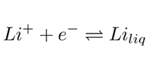
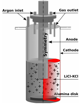
The demand for lithium has grown considerably during the last decades. Its importance has become unquestionable for the production of electronic devices and electric vehicles industry, where its lightweight and strong reduction potential is exploited. Batteries have been produced with a much higher volumetric and gravimetric energy densities - typically of the order of 160Wh/kg and 400Wh/L [1] - meaning almost 50% over conventional batteries. On the other side, lithium’s production presents some important technological difficulties, for instance the electrodes’ corrosion, back reactions, high energy demand, and the formation of unwanted foam [2–5]. Therefore, in order to optimize its production, modeling the behavior of a standard cell where lithium is produced by the electrolysis of LiCl, is an essential tool. Figure 1 shows a simplified schematic of a Li-production cell. At the cathode, Li⁺ reduces to its metallic liquid phase (Eq.1) eventually extracted from the cell as it floats on the electrolyte.

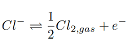
The oxidation of chloride takes place at the anode where bubbles are released (Eq.2), and their upward movement causes natural convection circulation of the liquid in turn.

A mathematical model of this electrolytic cell results in a strongly coupled set of partial differential equations representing the complex interactions between these physical phenomena. In the following, it is presented a solution to this strongly coupled mathematical model using an open-source CFD tool (OpenFOAM) that enables to address some of the simplifications that have been used in earlier works [6, 7]. The presence of the secondary phase (chlorine bubbles), its effect on the turbulence fields, and the liquid electrolytic flow circulation are taken into account as well as the effect of the tertiary current distribution. Therefore OpenFOAM is used here to accomplish the objective of this paper: showing for the first time to the authors knowledge the behavior of a Li electrolytic cell simulated with an OF model representing a two-phase turbulent flow, mass transfer in concentrated solutions (molten salt) and electrochemical surface reactions considering a tertiary current distribution.

2. Mathematical Modelling

The interaction among all phenomena just described is of utmost importance; however, for the sake of clarity, the governing equations below are split into three main areas of interest: fluid-dynamics, electrochemistry, and transport of ions.

2.1. Fluid-Dynamics

The bulk solution mainly consists of a liquid LiCl − KCl electrolyte, and a small amount of chlorine gas mostly located close to the anode. The cell dynamics obtained in a simulation without modeling the Cl_2,gas upward motion would be completely different, close to a common batch reactor. Therefore, a two phase Euler-Euler model is employed assuming that: only the drag force is relevant when compared to other interfacial forces [8]; bubbles are introduced with a constant size and spherical shape identified by the graphical scheme regime for bubbles and drops [9]; and the Schmidt number is fixed to 1.

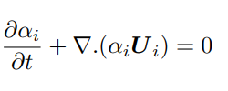
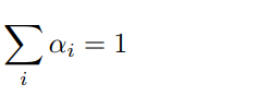
The Euler-Euler model [10] treats the two phases as continua, with a unique common pressure p [11]. It consists of one continuity equation (Eq. 3), a constraint equation on the sum of the two volume phase fractions α_i (Eq. 4), and one momentum equation per phase (Eq. 5):

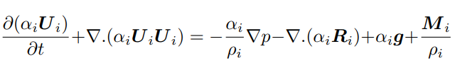
where the subscript i identifies the i_th phase, U the velocity, R the turbulent Reynolds stresses, and M the interfacial momentum transfer term considering the resistance force felt by each gas-bubble (Eq. 6)

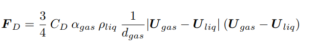
d_gas is the fixed bubble’s diameter, here set to 1.5 mm according to a similar experimental study [8], and C_D is the drag coefficient modeled as in Eq. 7 [12]:

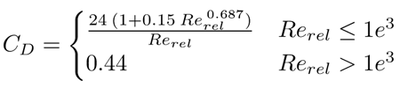
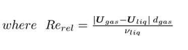
ν_liq is the liquid kinematic viscosity. The presence of the bubbles and their movement through the reactor promotes turbulence in the liquid phase, however due to their low concentration, the gas turbulence as well as the bubble-bubble collisions can be neglected [13]. Therefore the standard k − ε model is used only for the liquid phase as previously done in [14]. The model is chosen for its easy convergence, its robustness, and for performing well in the bulk of the flow. The balances of the turbulent kinetic energy (k), and the dissipation rate (ε) are expressed in Eq. 8 and Eq. 9:

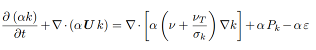
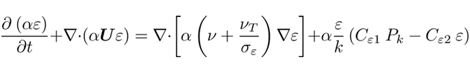
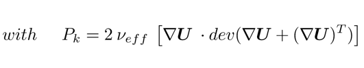
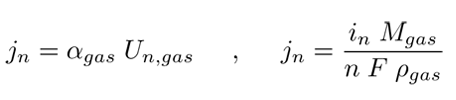
where the constants are C_ε1 = 1.44, C_ε2 = 1.92, σ_k = 1.0, σ_ε = 1.3, ν_eff is the sum of the laminar ν and turbulent viscosity ν_T, and P_k stands for the production of turbulent kinetic energy [10, 15–17]. The closure of this first set of equations comes with the appropriate boundary conditions shown in Table 1. At the anode the volume fraction of the gas, α_gas, depends on the distribution of the normal current density i_n and affects the normal mass flow rate j_n as shown in Eq. 11, [18]; meanwhile the pressure gradient is tuned according to the velocity to maintain a constant flux.

The turbulent variables k, ε, and ν_T follow the well known algebraic relations from literature [19–21], re-grouped in Table 1 where Ti is the turbulence intensity, and l_mix the turbulent mixing length. The cathode is treated as the bottom wall, and the wall functions, wf, solve the boundary layer for the turbulent variables [22]. The upper edge of the system is modeled as a free surface. Here a mixed boundary condition is imposed for both α_gas and U_gas, so that the gas can leave the system, while the liquid remains confined and controlled by a slip condition. The combination of these reproduces a degassing boundary condition [23].

Table 1. Fluid-dynamics boundary conditions with the OpenFOAM-nomenclature.

Variable	Anode	Cathode & Walls	Outlet
αgas		∇αgas = 0	inletOutlet
Un,gas	jn/αgas	no − slip	inletOutlet
Uliq	no − slip	no − slip	slip
p	∇p= fx(U)	∇p = fx(U)	fixedValue
k	1.5(Ti Uliq)2	wf	∇k = 0
ε		wf	∇ε = 0
νT	Cµk2/ε	wf	∇νT = 0

2.2. Electric Field and Current Distribution

The charges distribution between the electrodes is the result of the current conservation law shown in Eq. 12. The first term represents the ohmic contribution, basically the potential gradient times the electrolyte’s conductivity (later named K_e); while the second term is the polarization contribution.

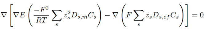
where the subscript s identifies the s_th species, T is the constant temperature of the ionic solution, z the charge number, C the ion’s concentration, F the Faraday’s constant, and E the electrolytic potential. Two additional variables appear in Eq. 12: the molecular diffusion coefficient (D_s,m) of the s_th species with respect to the total mixture modeled through Wilke’s correlation [24]; and the effective diffusivity (D_s,ef) arising from the turbulent and the molecular components (Eq. 13):

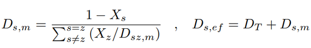
where X is the molar fraction, and the turbulent diffusion is modeled as D_T = ν_T.

The electrochemical boundary conditions are summarized in Table 2. At the anode the current applied faces both the kinetic contribution of the heterogeneous reaction and the overpotential of resistive layer due the freshly released bubbles. Therefore the slow oxidation of chlorine and the high overpotential are modeled through the Tafel approximation [25] considering an exchange current density of i_0,a = 10 A/m², and a symmetric coefficient of α_sym = 0.5. The high overpotential also reduces the concentration polarization contribution close to the electrode allowing a Neumann boundary condition for the electrolyte potential. On the contrary at the cathode the reduction of lithium is a fast reaction. The small overpotential allows the use of the linearized Butler-Volmer equation [25]. The exchange current density at the cathode is assumed to be high, for instance i_0,c = 1000 A/m², while the surface potential E_surf, and the equilibrium potential are set to zero, so that the whole cell potential is imposed at the anode. To conclude, the same slip boundary condition on the current density is imposed at the outlet and at the bottom wall.

Table 2. Electrochemical boundary conditions with the OpenFOAM-nomenclature.

Variable	Anode	Cathode
in
E

2.3. Transport of Ions

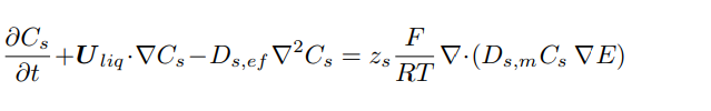
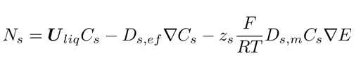
Inside this electrolytic cell, the movement of ions is driven by the electrolyte’s velocity (convection), the concentration’s gradient (diffusion), and by the potential’s gradient (migration). While the convection induces the same motion to all the species, the diffusive and the migrative mechanisms are dependent on the diffusion coefficients and the mobility of each species. The transport equation, Eq. 14, is solved for N_tot − 1 species, being Cl⁻, Li⁺, and K⁺ the modeled ions.

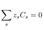
The extra equation needed to balance the number of unknowns is the electroneutrality of the solution, Eq. 15. It assures that there are no spurious charges floating around:

Note that there are no reactions in the bulk of the reactor, but only at the electrodes. The boundary treatments in Table 3 are expressed in terms of the fluxes N_s (Eq. 16), for clarity purposes. Nevertheless, in the source code mixed boundary conditions on concentrations are used instead. Those are implemented with blending functions weighting the Dirichlet conditions (migration term) and the Neumann conditions (diffusive term).

At the anode the only active species is the chloride. Its normal flux is regulated by Faraday’s law. Lithium and potassium ions do not react, and their flux is null. At the cathode a similar scenario occurs, but chlorine and lithium ions switch their roles. Lithium becomes the active species following the Faraday’s law, while chlorine do not react. The same condition as the anode holds for K⁺. A zero flux condition should be imposed for all species, but the migration term is already set to zero (Table 2), and the velocity at the wall is null. Therefore it is sufficient to impose a zero concentration gradient for all species.

Table 3. Concentration boundary conditions with the OpenFOAM-nomenclature.

Variable	Anode	Cathode

2.4. Simulation

Built using the framework of OpenFOAM, the numerical model developed uses an object-oriented approach, in which the classes’ structures are confined in specific regions of the code where they are easier to manage. The main core of the solver is made of two predictor-corrector loops, namely PIMPLE, and POTiso [26]. The PIMPLE algorithm takes care of the fluid-dynamics of the problem [27], [28], [29], [30], [31], and its biggest advantage is the increase of the time step without any restriction on the Courant number. Basically an initial guessed pressure is employed to solve the momentum equation and to get an estimation of the velocity. The latter is then used to update the pressure at the present time step, which in turn corrects the velocity. The solver also uses a Multidimensional Universal Limiter for Explicit Solution (MULES) method [32], to maintain boundedness of the phase fractions. Similarly, the electrochemical solver uses a predictor-corrector loop (POTiso) which starts with an initial guess on the potential, solves N_tot − 1 transport equations. The predicted species’ concentrations are then used to solve the charge continuity equation and get the updated value for the potential field. Finally the ions’ transport equations are solved again to correct their previous appraisals. The two loops are sequential since it can be assumed that there is a one-way-coupling between the fluid mechanics (advection) and the electrochemical phenomena [33].

All partial differential equations are solved using the Finite Volume Method. The first derivatives in time are discretized with an Euler first order, bounded, implicit method. The gradients are all discretized by means of the second order least squares method. The divergence terms are treated with a Gaussian second order, but they are of different types: a Gauss vanLeer is used in Eq. 3; a Gauss limitedLinearV 1 taking into account the direction of the field is used in Eqs. 5, 8, and 9, and finally a bounded upwind applies in Eq. 14. The laplacian schemes are handled with a Gauss linear corrected method, acting as an unbounded, second order, conservative method; and at last the interpolation schemes are simply linear. Furthermore all the boundary conditions are implemented through the utility groovyBC. For further details the reader is referred to the OpenFOAM user guide.

Additional information include:

• the initial composition of the concentrated solution consists of 60% of LiCl and 40% of KCl (molar basis)
• the bulk solution is in an isotherm equilibrium at 723 K
• a constant current of 65 A is imposed at the anode

The numerical domain illustrated in Figure 1 has the dimensions of 76 x 3.3 x 200 mm³, and it is divided in 4575 hexahedra cells, and 50 prisms, with a maximum skewness of 1.06. The wedge has an angle of 5^o.

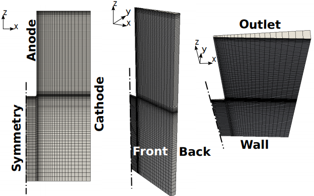
The maximum aspect ratio is 15, and it is located close to the corner of the L-shaped anode, where 4 refinement layers are applied to catch the exact amount of gas entering the system. Eight extra refinements are also added close to the Outlet, to make sure that the free surface is adequately approximated. The Wall and the Cathode present a coarser mesh so that the     y⁺ > 11 criteria [22] is respected and wall functions can be applied for the turbulent flow. The maximum mesh non-orthogonality is way below the critical value of 70, and its average is 6.9. The mesh just described is reported in Figure 2, and has positively passed the mesh dependency test explained in the Results section, proving that the solution is not affected by the mesh chosen. Analogously, a time dependency study has been carried out to assure that the simulations converge to the right solution in the shortest possible time. A time step of 1e⁻⁴ s has been selected. To solve the momentum equations for U, k, and ε a smooth solver is used, while the p is evaluated with a generalized geometric-algebric multi grid solver. The latter uses a coarse grid with fast solution times to shave high frequency errors and generate a starting solutions for the finer grid [34]. The conservation of charges makes use of a diagonal incomplete Cholesky preconditioned conjugate gradient solver. Finally the transport equations are solved through a diagonal incomplete LU preconditioned bi-conjugate gradient solver [32].

3. Results and Discussions

Before presenting the results of this work, a spatial grid convergence analysis is carried out to prove the independence of the results from the mesh size [35]. To do so, three meshes with a grid refinement ratio r of 1.6 are considered [36]; their characteristics can be found in Table 4. The order of convergence of the solution m is estimated via Eq. 17, by assuming the functional f to be the concentration of lithium integrated over the cathode surface. In this way the solutions of the fluiddynamics, the electrochemistry and the transport of ions are all verified in once.

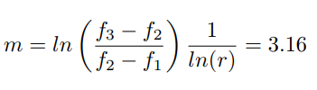
Table 4. Meshes used in the grid sensitivity analysis.

Grid ID	Number of cells	f
1	7400	0.02368
2	4625	0.02547
3	2890	0.03341

The real solution is then retrieved through the Richardson extrapolation [37] estimating f for a zero spacing grid as in Eq.18

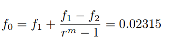
At this point one can calculate the discretization error also called Grid Convergence Index (GCI) in Eq.19, and if its value is less than 5% the solution is considered acceptable [35, 36].

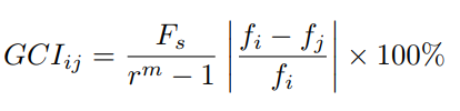
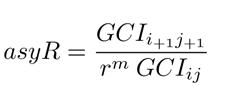
where F_s = 1.25 is a security factor. Finally an asymptotic range of convergence Eq.20 1 assures that the solution is within the error band

The spatial grid convergence analysis summarized in Table 5, points at the grid with ID 2 as the one to be used in terms of computational effort and accuracy.

Table 5. Results: Grid sensitivity analysis.

r	m	GCI12	GCI23	asyR
1.6	3.16	2.75	11.342	1.075

3.1. Fluid-Dynamics

The first predictor corrector loop solves the fluid-dynamics of the problem and the associated turbulence. Figure 3 shows the magnitude of the electrolyte’s velocity field after 3600 s. The peak of 0.291 m/s is found close to the anode where the gas, released by the oxidation of chloride, drags the electrolyte upward. Once the electrolyte reaches at the outlet, it can not escape (as imposed by its slip condition), and it is pushed rightward the cathode. Then it falls down and it is pulled back inside the bulk, where it splits in two parts: a faster clockwise re-circulation on the upper side of the cell, and a slower counterclockwise re-circulation at the bottom. On top of the colored magnitude velocity map, Figure 3 shows also the electrolyte’s velocity vectors. The vectors are not scaled with the velocity magnitude direction; the intent here is only to identify the direction of the flow and the zones just described.

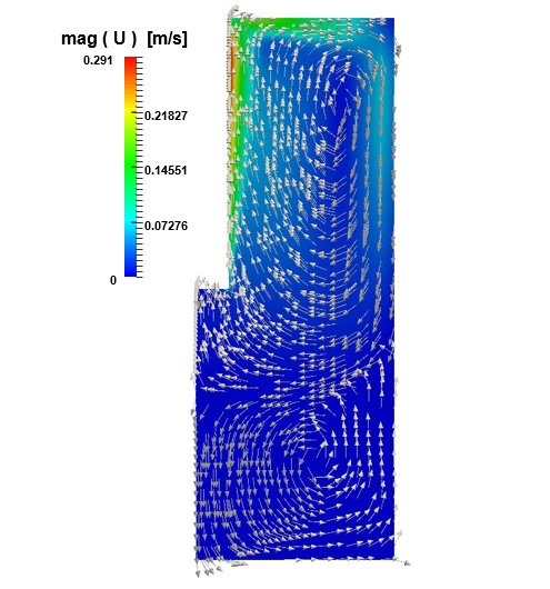
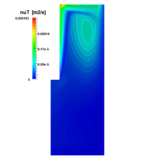
The same three zones can be identified in Figure 4. The peak this time is located at the upper end of the anode, where the flow changes sharply. The nucleus of the clockwise circulation is shifted with respect to the center of the electrodes’ gap, because a portion of the flow with lower kinetic energy is entrapped. Meanwhile the wall functions along the cathode and the bottom wall integrate appropriately the kinematic viscosity from the bulk through the viscous sub-layer.

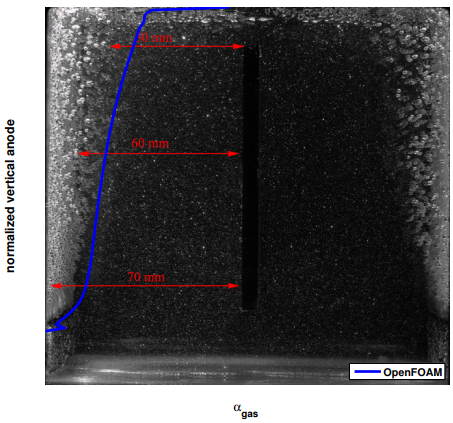
The induced gas velocity field map is not shown here since the Cl_2,gas remains confined to a thin layer close to the anode and escapes once it reaches the top of the cell. Very little gas can be seen at the free surface interface, but it does not affect the flow afterwards. On the other hand, the bubble coverage along the anode is much more of interest. Since the authors are not aware of available experimental measurements published on this type of cell configuration for lithium production, a magnesium cell with a similar behavior is used for the validation of the model. This cell has a slightly different configuration with two vertical parallel anodes, a cathode placed in between and an electrolytic solution with a fixed flow rate injected from the bottom [8]. After matching the initial conditions of the experimental data [8], the calculated gas distribution is plotted on top of the PIV data image in Figure 5 with the permission of the Canadian Journal of Chemical Engineering. The image shows in grey that the presence of bubbles is mostly concentrated close to the anodes and to the free surface. The blue line identifies the gas volume fraction (namely α_gas ) obtained in this work. After the initial small oscillation at the bottom entrance of the left anode, the curve follows the same behavior of the bubbles in the background of the image, showing that the present model appears to reproduce adequately the bubble’s movement. The red horizontal lines help to measure the growth of the bubble layer, being null at the entrance of the electrode, 10 mm in the middle, and increasing up to 20 mm close to the free surface.

3.2. Electrochemistry

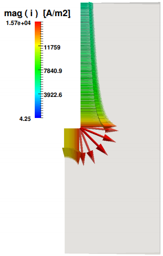
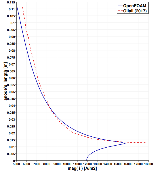
The second calculation loop solves the electrochemical part, whose results are described below. Figure 6 shows the magnitude of the current density vectors along the anode. The peak of 1.5e4 A/m² at the lower anodic corner decreases gradually toward the two other extremities of the electrode. The importance of this result is crucial since it is responsible for the gas velocity distribution, which in turns induces the electrolyte motion, which in turns affects the convective mechanism of the transported ions, and as a consequence the electric potential field. In Figure 7 the anodic current density resulting from this study is compared with the anodic current density of published work of Oliaii [6]. The ordinate measures the length of the whole anode, where the zero corresponds to the left extremity of the horizontal part and the value of 0.115 m to the last point at the top of the vertical anode. The peak is located at the corner between these two parts. The solid blue line is the result of this work, and the red dashed line is extracted from [6], where the horizontal contribution is not considered.

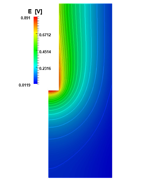
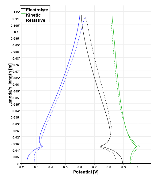
Analogously the electric potential field is reported in Figure 8. The maximum values are found at the bottom of the anode, where the bubble coverage is less as shown in Figure 5. Away from the anode, the electric potential decreases all the way down to the cathode, where only the kinetic overpotential is present. A more detailed description of the anodic scenario is plotted in Figure 9. The ordinates indicate the anodic length as explained for Figure 7, and the abscissa the intensity of the potentials expressed in [V ]. The solid lines are the results of this study, while the dashed lines reproduce the results of [6]. The black lines show the trend of the electrolytic potential.

Apart from a small portion of the electrode, its value decreases from the bottom of the vertical anode up to the top. The same occurs to the kinetic overpotential with the only difference being the concavity of the curve. An opposite behavior is noted on the distribution of the resistive overpotential induced by the gas film. Its lowest value is registered at the horizontal anode and it increases (almost linearly) all the way up to the outlet of the cell, where the resistive layer created by the bubble reduces the conductivity of the nearby electrolyte. All the three potentials present a peak at around 0.012 m, which corresponds to the corner of the L-shaped anode as already mentioned for the current density distribution.

3.3. Transport of Ions

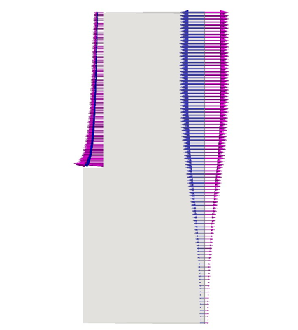
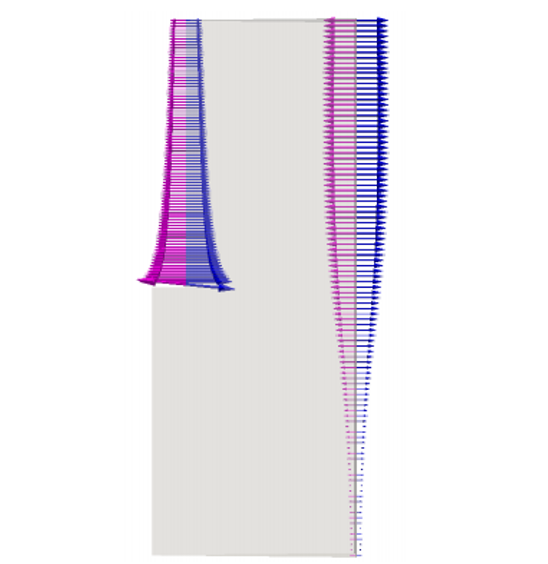
The last part of this section presents the fluxes of the three ions at the electrodes of the cell, describing the diffusion share (in magenta) and the migration share (in blue). The contribution of the convection at the electrodes is zero since a non slip condition is imposed for the electrolyte’s velocity.

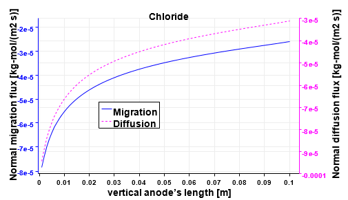
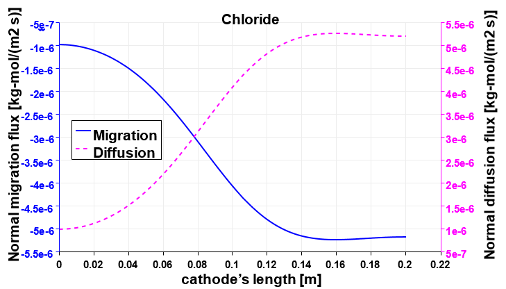
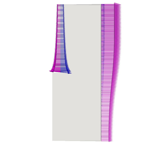
Figure 10 plots the perpendicular components of both the migration and the diffusion fluxes of Cl⁻. The horizontal part of the anode is not presented for the sake of clarity, but it follows the same trend as the vertical part. The arrows at the left electrode are scaled with the magnitude intensity of the vectors themselves; but a magnifying factor is applied on vectors at the right electrode to better check the direction of the fluxes at the bottom of the cell where their intensity is smaller. At the positive electrode both fluxes are exiting the domain. Figure 11 shows the monotonic trends of the anodic fluxes decreasing in an absolute value from 8e⁻⁵ kgmol/(m²s) at the anode’s corner, to approximately 3e⁻⁵ kgmol/(m²s) at to the outlet. It is important to point out that along the anode the two fluxes are not the same. Their sum is the result of the chloride’s heterogeneous reaction and it is proportional to ∼ i_n/(n_Cl− F) as described in Table 3. On the other hand at the cathode, chloride is a non-active species, and its total flux impacting the electrode has to be zero. Figure 12 proves that the contribution of the diffusion flux cancels out the migration component in each segment of the cathode. Additionally both cathodic curves change their curvature at approximately 0.08 m from the bottom of the cell. This is the location where the electrolytic flow splits into two counter rotating zones, affecting the turbulent diffusion and the effective diffusivity. It is also possible to notice that the fluxes on this side of the reactor present normal components one order of magnitude smaller than those at the anode as previously mentioned.

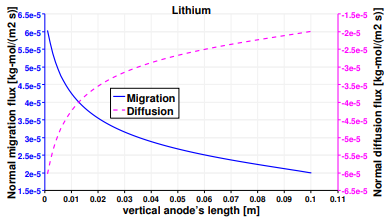
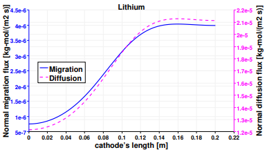
The same analysis is performed on lithium, and Figure 13 presents the normal vector components of its diffusive and migrative fluxes at the electrodes. The first main difference with respect to Figure 10, is the opposite direction of the migrative arrows, due to their charge number z_Li+ = −z_Cl−. Lithium ions are attracted to the positive electrode, and tend to escape the negative cathode. Despite the magnifying factor used for vectors at the negative electrode, the migrative contribution is still weak, especially at the bottom of the reactor. The anode represents the non-active surface for lithium, in fact the two fluxes have opposite directions and cancel each other. Figure 14 plots the normal diffusion and migration fluxes along the vertical anode, with the diffusive mechanism being predominant as it can be noticed on the right scale of Figure 15. The sum between the two fluxes is the results of the heterogeneous reaction occurring at the cathode (see Table 3). Nevertheless the shapes of the two curves are similar and their inflection point is again located around 0.8 m from the bottom of the cell.

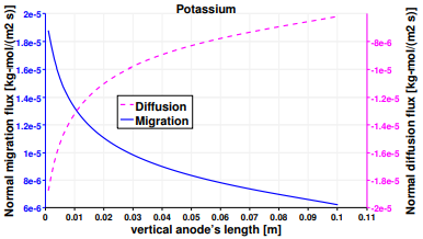
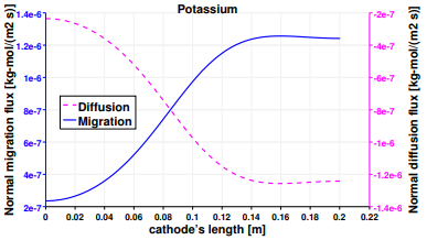
The study is completed by presenting the results of the mass transport of the third species, K⁺. Figure 16 reports that the migration fluxes of K⁺ are aligned with those of Li⁺ due to their equal charge numbers. Potassium is the only considered species which is non-active at both the electrodes. Indeed it presents the same fluxes’ behavior of Lithium at the anode and of Chloride at the cathode. Nevertheless their scales are not the same due to the different diffusion coefficients and concentration’s gradients of the species. Therefore, the same considerations elaborated before for Figures 12 and 14 are valid for Figures 18 and 17.

4. Conclusions

A mathematical model for an electrochemical cell is developed and solve numerically using the open-source CFD package OpenFOAM-2.3.1 to investigate the performances of a standard cell for the production of lithium in molten salts. Two predictor-corrector loops in series were used to first solve the fluid-dynamics equations and then the electrochemical equations. The electrochemical cell model takes into account the presence of the bubbles of chlorine released by the reaction at the anode and their effect on the flow of the liquid electrolyte. The upward movement of the gas due to their low density induces a natural convection on the electrolyte otherwise motionless. The flow becomes turbulent and a standard k −ε model is applied for the liquid phase. The steady state of the electrolytic flow presents three main zones: a fast zone close to the anode moving upward, a clockwise re-circulation on the upper side of the cell, and a counterclockwise re-circulation at the bottom. The electrochemical part solves the conservation of charges accounting for ohmic drop, concentration polarization, and also electrochemical kinetics. The distribution of current density along the anode shows a peak at the bottom corner. The same peak occurs on the electrolytic potential, the kinetic and the resistive overpotential. The latter reflects the presence of the film where the bubbles are mostly concentrated, reducing the overall conductivity of the electrolyte. The electrochemical aspect is validated by comparing the results of the present model to previously published studies [6]. The last part of this work focuses on the transport of ions and the results are presented in terms of fluxes. Results show that the normal migration flux cancels out the normal diffusion flux in presence of non-active species, while in case of active species the two contributions are summing up. The shape of all anodic fluxes report a similar trend to the current density, recalling the strong effect of the gaseous bubbles released by the oxidation of chloride. Analogously, the shape of all cathodic fluxes recalls the influence of the electrolytic flow with an inflection point located at ∼ 0.8 m from the bottom of the cell, where the flow splits into two counter rotating zones.

Acknowledgments

A special thanks goes to the Canadian company HydroQuebec, and to the NSERC which financially supported this study. The authors also thank the Université de Sherbrooke for its fellowship.

Nomenclature

Symbol	Units	Description
asyR	−	asymptotic range
CD	−	drag coefficient
Cε1,Cε2	−	empirical turbulent constants
Cl−	−	chlorine ions
Cl2,gas	−	chlorine gas
Cµ	−	empirical turbulent constant
Co	−	Courant number
C		concentration
Ds,ef		effective diffusion coefficient
Ds,m		molecular diffusion coefficient
DT		turbulent diffusion coefficient
dgas	m	bubble’s diameter
E	V	electric potential
Esurf	V	surface potential
	V	equilibrium potential
F		Faraday’s constant
FD		drag force
Fs	−	security factor
f	−	functional
GCI	−	Gric Convergence Index
g		gravity vector
i0,a,c		exchange current density
in		normal current density
jn		specific normal mass flow rate
K+	−	potassium ions
Ke		electrolyte conductivity
k		turbulent kinetic energy
Li+	−	lithium ions
Liliq	−	liquid lithium
lmix		turbulent mixing length
Mi		interfacial momentum transfer
Mgas		molar mass of the gas phase
m	−	order of convergence
N		flux of ions
Ntot	−	total number of species
n	−	number of electrons reaction

Symbol Units		Description
PIV	−	Particle Image Velocimeter
Pk		k production
		pressure
R		gas constant
Ri		turbulent Reynold stresses
r	−	grid refinement ratio
Rerel	−	relative Reynolds number
T	K	temperature
Ti	−	turbulent intensity
t	s	time
U		velocity vector
Un		normal velocity component
uτ		friction velocity,
Xs	−	molar fraction
wf	−	wall functions
y	m	wall distance
y+	−	non dimensional wall distance,
z	−	charge number

Greeks	Units	Description
αi	−	volume fraction
αsymm	−	symmetry coefficient fixed to 0.5
	V	overpotential
νeff		effective kinematic viscosity
νliq		liquid kinematic viscosity
νT		turbulent kinematic viscosity
ε		turbulent dissipation rate
ρgas		density of the gas phase
ρi		density
σk	−	empirical turbulent constant
σε	−	empirical turbulent constant
τw		wall shear stress, µ(∂yU)|w

References

[1] T. B. Reddy and D. Linden, Linden’s Handbook of Batteries, fourth edition, 4th ed. Mc Graw Hill, 2011.
[2] E. S. McCormick, S. S. Reddy, and K. Sintim-Damoa, “Electrolytic production of lithium metal,” U.S. Patent 4455202, 1984.
[3] D. DeYoung, “Production of lithium by direct electrolysis of lithium carbonate,” U.S. Patent 4,988,417, Jan. 29, 1991. [Online]. Available: https://www.google.com/patents/US4988417
[4] W. H. Kruesi and D. J. Fray, “Fundamental study of the anodic and cathodic reactions during the electrolysis of a lithium carbonate-lithium chloride melt using a carbon anode,” Journal of Applied Electrochemistry, vol. 24, no. 11, pp. 1102-1108, 1994. [Online]. View Article
[5] S. Amendola, L. Swonger, and S. Goldman, “Electrolytic production of lithium metal,” U.S. Patent App. 13/172,401, Jan. 12, 2012. [Online]. Available: http://www.google.com/patents/US20120006690
[6] E. Oliaii, M. D´esilets, and G. Lantagne, “Numerical analysis of the effect of structural and operational parameters on electric and concentration fields of a lithium electrolysis cell,” Journal of Applied Electrochemistry, vol. 47, no. 6, pp. 711-726, 2017. View Article
[7] F. Rivera, C. Ponce de Le´on, J. Nava, and F. Walsh, “The filter-press fm01-lc laboratory flow reactor and its applications,” Electrochimica Acta, vol. 163, pp. 338-354, 2015. View Article
[8] C. L. Liu, G. M. Lu, X. F. Song, and J. G. Yu, “Experimental and numerical investigation of two-phase flow patterns in magnesium electrolysis cell with non-uniform current density distribution,” The Canadian Journal of Chemical Engineering, vol. 93, pp. 565-579, 2015. View Article
[9] R. Clift, J. R. Grace, and M. E. Weber, Bubbles, drops, and particles, Academic Press, New York-San Francisco-London, 1978.
[10] H. Rusche, “Computational fluid dynamics of dispersed two-phase flows at high phase fractions,” Ph.D. Thesis, Imperial College of Science, Technology and Medicine, UK, 2002.
[11] G. Holzinger, Openfoam a Little User-Manual, CDLaboratory - Particulate Flow Modelling Johannes Keplper University, Linz, Austria, 2015.
[12] L. Schiller and Z. Naumaan, “A Drag Coefficient Correlation,” V.D.I Zeitung, vol. 77, p. 138, 1935.
[13] I. ANSYS, Fluent theory guide, 14.0 ed, 2011.
[14] G. Litrico, C. B. Vieira, E. Askari, and P. Proulx, “Investigation of the optimum operative conditions for a parallel plate electrochemical reactor,” ECS Transactions, vol. 75, no. 37, 2017. View Article
[15] D. Wilcox, Turbulence Modeling for CFD. La Canada, CA: DCW industries, 1993.
[16] S. Pope, Turbulent Flows. Lancaster, New Jersey: Cambridge University Press, 2000.
[17] J. Mathieu and J. Scott, “An introduction to turbulent flow,” Cambridge University Press, 2000.
[18] A. Alexiadis, M. Dudukovic, P. Ramachandran, A. Cornell, J. Wanngard, and A. Bokkers, “Liquid-gas flow patterns in a narrow electrochemical channel,” Chemical Engineering Science 66, vol. 66, pp. 2252-2260, 2011. View Article
[19] H. Tennekes and J. L. Lumley., A first course in turbulence, Massachusetts Institute of Technology, 1999. View Book
[20] M. Lesieur, Turbulence in fluids, 4th edition, Springer, 2008.
[21] P. A. Libby, Introduction to Turbulence, Taylor and Francis, 1996. View Book
[22] H. Schlichting and K. Gersten, “Boundary-layer theory, 9th edition,” Springer, 2017. View Book
[23] X. Miao, D. Lucas, Z. Ren, S. Eckert, and G. Gerbeth, “Numerical modeling of bubble-driven liquid metal flows with external static magnetic field,” International Journal of Multiphase Flow, vol. 48, pp. 32-45, 2013. View Article
[24] D. F. Fairbanks, C. R. Wilke “Diffusion coefficients in multicomponent gas mixtures,” Industrial and engineering chemistry, vol. 42, no. 3 ,1950. View Article
[25] J. Newman, K. Thomas-Alyea, Electrochemical Systems, 3rd Edition, John Wiley and Sons, New Jersey, 2004. View Book
[26] G. Litrico, C. B. Vieira, E. Askari, and P. Proulx, “Strongly coupled model for the prediction of the performances of an electrochemical reactor,” Chemical Engineering Science, vol. 170, 2017. View Article
[27] R. Issa, “Solution of the implicitly discretized fluid flow equations by operator-splitting,” Journal of Computational Physics, vol. 62, pp. 40-65, 1985. View Article
[28] R. Issa, A. Gosman, and A. Watkins, “The computation of compressible and incompressible recirculating flow by a non-iterative implicit scheme,” Journal of Computational Physics, vol. 62, pp. 66-82, 1986. View Article
[29] H. Jasak, “Error analysis and estimation for the finite volume method with applications to fluid flow,” Ph.D. Dissertation, Imperial College of Science, Technology, and Medicine, Department of Mechanical Engineering, 1996, pp 146-152. View Article
[30] P. Oliveira and R. Issa, “An improved piso algorithm for the computation of buoyancy-driven flows,” Numerical Heat Transfer, vol. 40, pp. 473-493, 2001, part B. View Article
[31] J. Ferziger and M. Peric, Computational Methods for Fluid Dynamics, 3rd ed. Springer-Verlag, 2002, pp. 176.
[32] OpenFoam, The Open Source CFD Toolbox, User Guide, 2014.
[33] M. Rosales and J. Nava, “Simulations of turbulent flow, mass transport, and tertiary current distribution on the cathode of a rotating cylinder electrode reactor in continuous operation mode during silver deposition,” Journal of The Electrochemical Society, 2017. View Article
[34] T. Behrens, “Openfoam’s basic solvers for linear systems of equations,” Chalmers, Department of Applied Mechanics, Technical report [Online], 2009. View Report
[35] J. Slater, “Examining spatial (grid) convergence,” 2008. [Online]. Available: https://www.grc.nasa.gov/www/wind/valid/tutorial/spatconv.html
[36] P. Roache, Verification and Validation in Computational Science and Engineering, New Mexico. Hermosa Publishers, 1998, pp. 358-359.
[37] L. Richardson, “IX. The approximate arithmetical solution by finite differences of physical problems involving differential equations, with an application to the stresses in a masonry dam,” Philosophical Transactions of the Royal Society of London A: Mathematical, Physical and Engineering Sciences, vol. 210, no. 459-470, pp. 307–357, 1911. [Online]. Available: http://dx.doi.org/10.1098/rsta.1911.0009