Journal of Fluid Flow, Heat and Mass Transfer (JFFHMT)

ISSN: 2368-6111

Introduction

The pulp and paper industry accounts for more than half of the energy consumed by the entire Swedish manufacturing sector [1]. However, the industry is also a large producer of energy. Data from 2012 show that the energy production from biological residue amounted to 42.3 TWh in that year [2]. Improving energy efficiency by a small percentage can thus save large amounts of energy, and large reductions could even in the long-term lead to the industry becoming net exporters of green energy.

The disc refiners, where fibres are mechanically processed, are a very energy intensive part of the production line. The energy consumption for a single disc refiner can be more than several megawatts [3]. The basic design of a disc refiner is a rotating disc at a close distance from a static disc, where the surfaces of the discs are patterned with bars. Fibres are fed through the centre of the discs and forced to the outer diameter. Research indicates that this process creates cavitation inside the disc refiners [4]. Cavitation is generally unwanted as it causes mechanical wear on the refiners. However, there may also be positive effects as cavitation can increase the fibrillation of the fibres [5].

1.1. Proposed Future Design

An entirely novel technology for fibre refining, which could significantly lower the energy consumption in this part of the process, was suggested by Johansson and Landström [6]. Instead of viewing cavitation as an undesirable by-product, the power of the bubble collapse could be utilized for the fibrillation and processing of pulp fibres. Cavitation can be induced in a few different ways: by hydrodynamics, by ultrasound or by a combination of the two. Hydrodynamic cavitation has the lowest energy consumption of the three [5] and can be achieved by running the pulp stream through a venturi nozzle. The cavitation bubbles will collapse when the pipe expands and the static pressure recovers. The idea is to focus the bubble collapse on the surface of the fibres to achieve fibrillation and processing.

1.2. Project Outline

The pulp processing concept was studied numerically using numerical simulations in three phases, see the project outline in Table I. First an optimal venturi shape was determined using 2D simulations and a recently developed optimization method. The optimal shape was then validated using a more detailed 3D simulation. These initial simulations were performed on a pure water flow. Finally, the effects of fibres in the pulp suspension were included and the onset of cavitation was investigated in a series of detailed 3D simulations.

2. Phase 1: Optimization of Venturi Shape

An optimal venturi configuration was determined using a recently developed optimization method [7,8]. The method is a two-level optimization method, meaning that the optimization is performed on a solver approximation instead of the full solver. In short, the method generates a number of venturi configurations within specified parameter limits using Latin Hypercube Sampling (LHS). Numerical simulations are run on these configurations and an approximation of these simulations is created using neural networks.

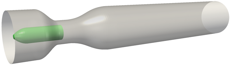
An optimal configuration is determined from this neural network solver approximation using an evolutionary optimization method. For details the reader is referred to [8]. The venturi nozzle concept is shown in Figure. 1, rotated to fit the page.

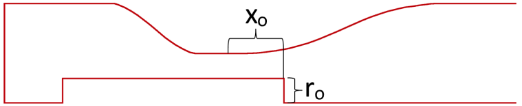
The inlet is located at the bottom (left in the figure) with flow upwards (to the right in the figure). The concept includes an obstruction object located in the venturi throat. A broad parameter study on the venturi nozzle covering four geometrical parameters as well as inlet and outlet pressure was performed in [8]. This investigation was used as input for a more detailed investigation covering two geometrical design parameters, obstruction radius r_o and obstruction position x_o, as well as inlet pressure P_in. The problem is axisymmetric and numerical simulations were performed on the 2D model shown in Figure 2.

The aim of the optimization was to achieve a design where cavitation was initiated and sustained in the centre of the venturi and to avoid cavitation at the walls. Volume fraction of vapour was used as a measure of cavitation. The simulations were performed in Fluent using a transient URANS turbulence model and the Schnerr-Sauer cavitation model. Vapour fraction was computed as the time average in two zones, a centre zone and near-wall zone shown in Figure. 3. The optimization aimed at maximizing vapour fraction in the centre zone and minimizing vapour fraction in the near-wall zone.

The parameter study yielded an optimal configuration with 17.3% vapour fraction in the centre zone and 0.8% in the near-wall zone. The optimal venturi parameters and their respective limits are presented in Table II.

Table 1. Project outline. The simulations were separated into three phases.

Phase	Aim	2D	3D	Fiber modelling	Simulation complexity
1	Optimization of Venturi shape	X
2	Validation of optimal venture shape		X
3	Investigation of cavition onset		X	X

Table 2. Optimal venturi nozzle parameters. Obstruction radius and position are reported relative to the throat radius, R_t.

Phase	Parameters			Vapour fraction
	r0	x0	Pin	Centre	Wall
Optimal	0.62Rt	-0.19 Rt	3.00 bar	17.3%	0.8%
Min	0.30Rt	-0.20 Rt	3.00 bar	--	--
Max	0.70Rt	-0.40 Rt	3.00 bar	--	--

3. Phase 2: Validation of Optimal Venture Shape

A 3D numerical simulation was run to validate the optimal configuration shown in Table II. The simulation was performed on a quarter model (90°) of the venturi in order to reduce the computational time. The open boundaries of the channel were treated as symmetry planes.

3. 1. Solver

The simulations were performed in Fluent, using a coupled pressure-based solver. Phase interaction was modelled with the mixture model and cavitation was modelled with the Schnerr-Sauer model. Turbulence was modelled using a hybrid LES/RANS model called Detached Eddy Simulation (DES). The flow was first solved using a steady RANS model, before switching to the transient DES model. The time step was set to result in a maximum CFL number of 1, as recommended for the turbulence model [9]. The simulation temperature was set to 72°C (345 K) as this was considered a representative temperature for the pulp processing. The inlet pressure was set to 3.0 bar as determined in the 2D optimization. The outlet pressure was similarly set to 1.0 bar.

Results were post-processed using the open source software ParaView. The initial numerical fluctuations were disregarded and results were time-averaged once the solution had stabilized.

3.2. Limitations

All simulations were performed on a pure water flow instead of a fibre suspension in order to reduce the complexity of the simulations. A pure water flow also means that there is no solute gas in the water, a parameter which affects the amount of cavitation bubbles. This is however accounted for in the cavitation model, which assumes an abundant supply of cavitation nuclei and is therefore not considered a limitation. The average vapour fraction in each zone for the 2D optimization and 3D validation is listed in Table III. A visual comparison is presented in Figure. 4.

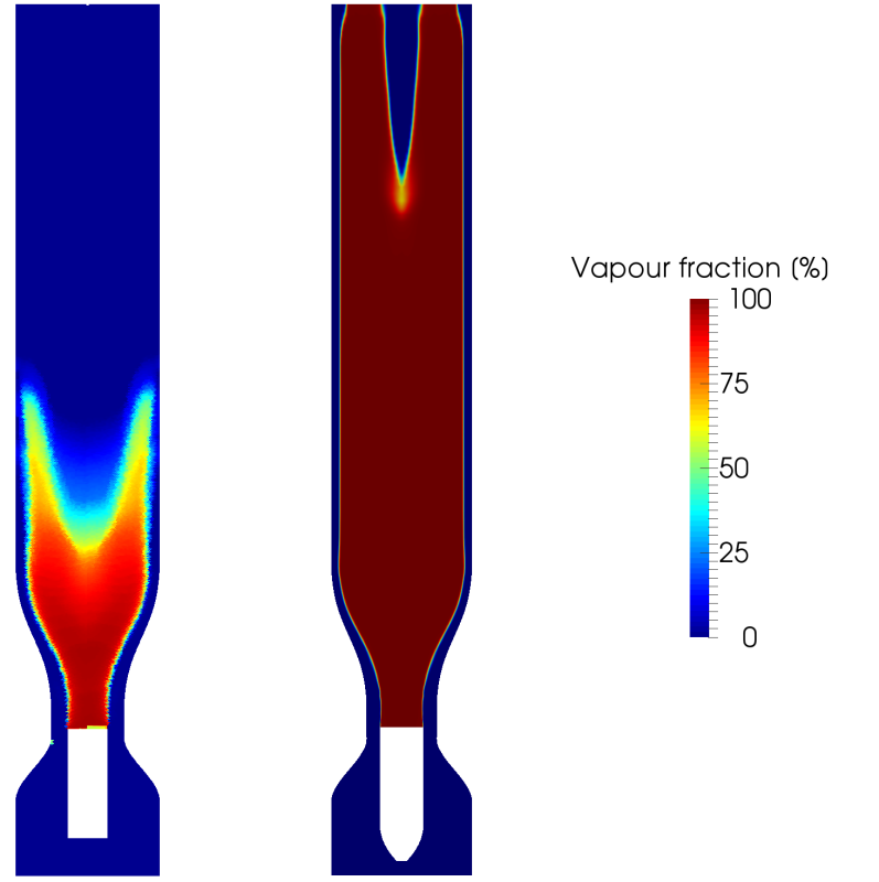
Table III shows that the vapour fraction values of the 3D validation do not match the values of the 2D optimization. This is also confirmed in Figure. 4. The 3D simulation yields both a higher vapour fraction in the centre of the channel and a lower vapour fraction near the wall. The difference is probably related to the limitations found in the cavitation model, see section IV below. The results of the 3D validation do however show that the aims of the optimization have been achieved, with an almost maximum vapour fraction in the centre of the channel and a minimum vapour fraction near the wall.

4. Limitation in the Cavitation Model

During the 3D validation simulations, there were large issues with pressure fluctuations in the channel. These instabilities would occur only after the simulations had run for a while. This was first assumed to be a problem related to the mesh or some model settings. After many tests and contact with ANSYS’ cavitation specialists this was confirmed to be a previously unknown bug in the cavitation modelling in Fluent. The problem was found in both tested cavitation models, Schnerr-Sauer and Zwart-Gerber-Belamri. In their current state, the cavitation models in Fluent are therefore not suited for shear cavitation (cavitation generated in the wake behind a bluff body as opposed to wall cavitation), which is the application investigated in the current project. As a consequence, the cavitation models could not be used for subsequent simulations. In effect, the possibility to predict the lifespan of cavitation bubbles disappeared. However, it was still possible to investigate the critical conditions for the onset of cavitation. Cavitation can occur when the minimum pressure is below the vapour pressure, i.e.

Table 3. Comparison of average vapour fraction in each zone for 2D optimization and 3D validation.

Zone	Optimization aim	2D Optimization	3D validation
Centre	100.0%	17.3%	99.0%
Wall	0.0%	0.8%	0.0%

Incipient conditions for cavitation is defined as the limit where . This is not a definitive limit for cavitation, but merely an indication. Other effects, such as surface tension, could delay the onset of cavitation. But as stated in [10] the vapour pressure limit is good approximation for the onset of cavitation, particularly in industrial applications.

5. Phase 3: Investigation of Cavitation Onset

 A detailed investigation on the critical pressure conditions in the venturi for the onset of cavitation was carried out on the optimal venturi shape determined in phase 1 and 2. The simulations in large followed the solver setup used for phase 2, with two important changes. For the first, a fibre model was introduced to include the effects of the fibres in the pulp suspension. Secondly, the cavitation model was removed since it was determined to not be suitable for shear cavitation, see section IV. Instead the incipient conditions for cavitation was determined using (1).

5. 1. Fiber Modelling

A detailed study on fibre modelling for low-consistency pulp applications was recently conducted in [11]. It was concluded that, for fully turbulent flows, it is sufficient to use a simple Bingham model in order to capture the macroscopical effect of fibres on the flow. The method used is based on introducing a transport equation for fibre concentration and using a rheological model to update the fibre solution viscosity.

5.1.1. Bingham Model

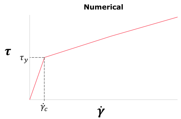
A method to numerically model fibre suspension flow with the Bingham viscoplastic fluid model and its implementation is described below. The yield stress for the suspension has been computed using the empirical relation

where  and  are model constants, varying from suspension to suspension, and is the mass concentration, or mass consistency, of fibres. In the theoretical case for a Bingham viscoplastic fluid the effective viscosity is infinite for shear stress levels below the yield stress. In a numerical model this may be approximated by assigning a large value to the viscosity for low shear rates and vary it linearly with shear rates corresponding to stress levels exceeding yield stress. That methodology, however, gives a discontinuity in the derivative  which may cause numerical issues. As specified in Fluent [9], suspension viscosity is computed as

where is consistency index which is equal to the viscosity of water, is critical strain rate, corresponding to the limit case were fluid shear stress equals the yield stress, and is computed as

And the constant  is set to a large value. Equation (3) was used to compute the viscosity of the fibre suspension for the Bingham model also in this thesis work. It can observed that the derivative of the viscosity with respect to shear rate yields

and is thus continuous, which also corresponds to a continuous derivative . A comparison between the numerical model for the viscosity with discontinuous derivative and the modified version is illustrated in Figure 5.

The above model was implemented and used for validation with experimental data to evaluate if the use of the same is justified or not. To make it possible to use the model alongside turbulence models in Fluent the suspension viscosity was instead computed in each cell from Equation (3) using a User Defined Function(UDF).In the flow model described an additional transport equation was introduced to account for local variations in fibre mass concentration , reading

where  is fibre concentration diffusivity. In this work, however, this transport was excluded. Both the cases for homogenous concentration in the whole domain and the case of non-homogeneous inlet concentration together with the use of Equation (6) was tested. It was found that both cases yielded practically the same simulation results. Solving Equation (6) would therefore solely raise the computational cost and it was therefore concluded that the fibre concentration may and should be treated as homogeneous.

5. 2. Estimation of Critical Cavitation Conditions

The 3D validation showed a large fraction of vapour in the channel, meaning that the onset of cavitation occurs at a lower pressure drop than this. The intensity of the bubble collapse depends on the surrounding pressure, where a higher surrounding pressure gives a more powerful bubble collapse. It is therefore preferable to decrease the pressure drop by increasing the outlet pressure rather than decreasing the inlet pressure.

A pressure sweep was performed on a rough mesh in order to estimate the critical pressure drop for the onset of cavitation. The pressure sweep included four different outlet pressures: 1.0, 1.3, 1.6 and 2.0 bar. The mesh, shown in Figure. 6, was created in ANSA and consisted of approximately 300,000 cells. It included boundary layers adapted for the DES turbulence model.

The minimum average pressure in the flow for the four outlet pressures is presented in Figure. 7. The pressure is measured behind the obstruction object, where cavitation occurred in the previous simulations. A linear regression of the minimum pressure is also included in the figure, as well as standard deviation and saturation pressure.

As can be seen in the figure the minimum average flow pressure at an outlet pressure of 1.5 bar corresponds well to the saturation pressure. Since the flow is turbulent the minimum pressure fluctuates around this value. Assuming that the minimum pressure has a normal distribution around the mean value (i.e. the linear regression), the minimum pressure would statistically be below the saturation pressure 50% of the time at this outlet pressure. This would constantly generate cavitation and could hardly be called incipient conditions.

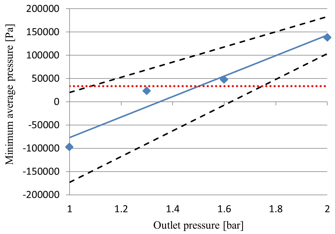
A better estimate is one standard deviation below the mean value, i.e. the bottom dashed line in Figure. 7. This line intersects the saturation pressure at an outlet pressure of around 1.7 bar. At this point the minimum pressure would statistically be below the saturation pressure around 16% of the time. This is of course not an exact definition of incipient conditions, but a good estimate.

5. 3. Detailed Simulation at Incipient Condition for Cavitation

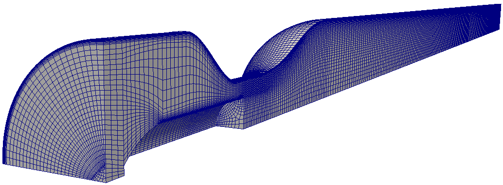
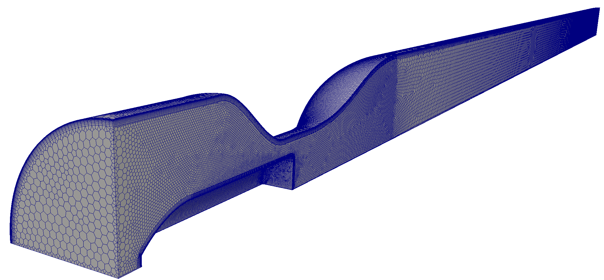
 A detailed simulation was run for the estimated incipient condition, i.e. at an outlet pressure of 1.70 bar. This was found to be a too low, so a second simulation was run with an outlet pressure of 1.90 bar. These detailed simulations were run on a much finer mesh than in the estimation pressure sweep. The mesh elements were also changed to polyhedral cells. The boundary layers were improved and boundary layers were also added to the obstruction object. The mesh, shown in Figure. 8, was created in ANSA and consisted of approximately 1.2 million cells.

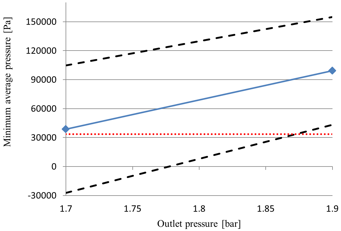
The minimum average pressure in the flow for the two simulations is presented in Figure. 9. A linear regression of the minimum pressure is also included in the figure, as well as standard deviation and saturation pressure.

The average pressure behind the obstruction object is very close to the saturation pressure for the simulation with an outlet pressure of 1.70 bar. However, once again assuming that the pressure is normally distributed around the average value, this would mean that pressure would be below the saturation pressure about 50% of the time. As stated in section V, subsection B, a better estimate of incipient conditions is one standard deviation below the mean value, i.e. the bottom dashed line in Figure. 9. This estimate would give a desired outlet pressure of 1.87 bar.

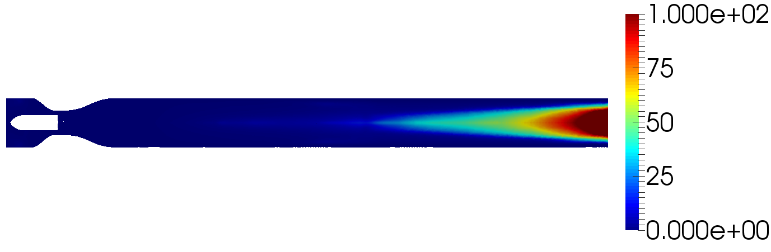
The fibre model couples the fibres and the flow by modifying the laminar viscosity. Figure. 10 shows the average laminar viscosity for the simulation. It can be seen that a portion of the flow is at or above the specified upper limit, which is set to 100 Pa∙s. This is the value of μ0 in (3) used in the fibre model and indicates the breakpoint in the Bingham model where the fluid starts flowing. In this case, it indicates the presence of a plug flow at the end of the channel.

An innovative concept for refining pulp using hydrodynamic cavitation has been investigated. A venturi nozzle has been designed and successfully optimized to initiate cavitation in the centre of the channel and to avoid cavitation at the wall. The optimal venturi shape was investigated in a series of detailed numerical simulations. The simulations used a Bingham fibre model to include the effect pulp fibres has on the flow. The investigation showed that cavitation bubbles start to form at an outlet pressure of 1.87 bar, for an inlet pressure of 3.00 bar. The intensity of the bubble collapse depends on the surrounding pressure and the determined outlet pressure therefore enables a powerful treatment of the pulp fibres. During the project it was found that the Schnerr-Sauer and Zwart-Gerber-Belamri cavitation models in Fluent are not suitable for shear cavitation. An investigation of the lifetime of cavitation bubbles was therefore not possible.

In conclusion, the venturi concept for processing pulp is plausible and seems promising at this stage. More research, in particular physical experiments, is however required before a conclusive verdict can be given. The initial focus of such experiments should be to measure the processing effect on pulp fibres and to make sure that no cavitation occurs at the venturi walls.

6. Conclusions

Approaches for modelling of turbulent fibre suspension flow were studied and successfully implemented numerically. The model was effectively acts as single-phase flow models through modification or addition of viscous stresses in the Navier-Stokes equation. The Bingham model, the suspension is modelled as a non-Newtonian fluid by computing the effective viscosity as a function of shear rate.

The model simulation results were compared to experimental data for validation. The parameter settings yielding the results with best resemblance of experimental data for the model were then identified. The model performed well along with reasonable computational cost and stability. The Bingham model had a simple implementation process. The Bingham model was therefore identified as the best model and was also used to simulate the flow in a disc refiner model and successfully resembled general flow patterns from numerical and physical experiments in literature. In summary the aim of the work was fulfilled, and a suitable fibre model was delivered.

7. Acknowledgment

The project has been carried out in collaboration with Åforsk, Energimyndigheten (Swedish Energy Agency), Luleå University of Technology, Holmen, SCA and Stora Enso.

References

[1] Swedish Energy Agency, “ET2013:22 Energiläget 2013 (Government report),” 2013.
[2] Statistics Sweden, “Industrins årliga energianvändning 2012 (Government report),” 2014.
[3] M. Illikainen, E. Härkönen, M. Ullmar and J. Niinimäki, “Power consumption distribution in a TMP refiner: comparison of the first and second stages,” TAPPI Journal, vol. 6, no. 9, pp. 18-23,2007. View Article
[4] O. Eriksen and L. Hammar, “Refining mechanisms and development of TMP properties in a lowconsistency refiner (Technical report),” Trondheim: Paper and Fibre Research Institute (PFI), 2005. View Article
[5] P. R. Gogate and A. B. Pandit, “Hydrodynamic cavitation reactors: a state of the art review,” Reviews in Chemical Engineering, vol. 17, no. 1, pp. 1-85, 2001. View Article
[6] Ö. Johansson and L.-O. Landström, “Slutrapport: Hur kan resonansfenomen utnyttjas för att minska energiförbrukningen vid framställning av papper (Technical report),” Stockholm: ÅForsk, 2010.
[7] A. Lundberg, P. Hamlin, D. Shankar, A. Broniewicz, T. Walker, C. Landström, “Automated aerodynamic 8 vehicle shape optimization using neural networks and evolutionary optimization,” SAE International Journal of Passenger Cars - Mechanical Systems, vol. 8, no. 1, 2015.
[8] K. Frenander, “Optimization and automated parameter study for cavitating multiphase flows in venturi - CFD analysis (Master's thesis)”, M.S. Thesis, Chalmers University of Technology, p. 61, 2014. View Article
[9] ANSYS Fluent theory guide (manual). ANSYS Inc., Canonsburg, PA, USA, 2013.
[10] J.-P. Franc, “Physics and control of cavitation. Design and analysis of high speed pumps,” Neuillysur-Seine, France: RTO, pp. 2-1–2-36, 2006.
[11] S. Ingelsten, “Fibre modelling in venturi flow and disc refiner – implementation and development of models for turbulent fibre suspension”, M.S. Thesis, Gothenburg: Chalmers University of Technology, 2015.