Journal of Fluid Flow, Heat and Mass Transfer (JFFHMT)

ISSN: 2368-6111

1. Introduction

Flow induced vibration (FIV) might draw attention people who care in engineering disciplines.  Even though the flow velocity runs out in a uniform direction, the D- Section, which was prepared in this experiment and subjected to various flow velocities and was sat up in various attack angles in front of fan tunnel, is non-symmetric.

Many of the previous papers regarding the flow induced vibration. The tunnel of wind was used to experiment flow induced vibration of an elastic circular cylinder by Brika and Laneville (1999) [1]. The system which is consisted of one degree of freedom is circular, but the system is fixed with a ridge which is added on the surface of the body. The ridge is used to transfer small vibration amplitude that is called a galloping, as suggested by A.H.P. van der Burgh, Hartono (2004) [2].

The one degree of freedom systems are variety of cross section area, so all issues regarding a galloping should be discussed. One of studies has been finished regarding damping parameters of one degree of freedom.  The damping parameters, which is represented as , are very important in practical aspect for VIV response prediction of elastic structure, investigated by J. Kim Vandiver (2012) [3].

In this work, the cylinder is mounted by the spring as the canonical issue that could be used to create comparison between the suggested alternatives and with the performance of variables of mass damping, studied by Govardhan and Williamson (2006) [4], Khalak and Williamson (1999) [5] and Klamo et al. (2005) [6].

2. Analysing for Flow-Induced Vibration simulation

In this part, the D- section system was simulated based on the shape properties and the materials components type which were used to manufacture it. The D-section system is consisted of one mass and viscous damping and a stiffness.

The properties of materials are one of the most important things to be taken consideration, because the properties of materials will be used to find certain variables of single degree of freedom (SDOF), which were subjected to various velocities. Whereas the derivation of equation of motion for D-Section plays a big role to simulate the system. On the other word, it could be impossible to simulate a system without knowing its equation of motion and analysing system of force directions.

2.1. The Geometrical Properties and Material Properties

The dimensions and material properties are one of the most important characteristic which are used to simulate the model, so the dimensions and material properties should have been found before starting with an experiment and a simulation for the model.

In this paper, the model is the D-Section which is consisted of polystyrene (C8H8)n as a mass with a steel as the viscous damping coefficient c and spring stiffness k, so the calculations of mass and stiffness for the D-Section should be finished by using the geometrical properties to these materials and the material properties of the body. Hence, and after searching about material characteristics for this model, it is found that the D-Section materials components are a steel and polystyrene (C8H8)n. the main material properties of the model, which were used to solve one issue or more than one in this paper, are Young's modulus E and the density .

Table 1. Shown the Geometrical Properties for polystyrene (C8H8)n as a mass and a steel as the viscous damping coefficient c and spring stiffness k.

Geometrical Properties	The mass	The spring
Length	L=28.2 cm	L= 20cm
Diameter, or width	D = 8 cm	b=38.45mm
thickness	-	h=1.06 mm
Material Properties	The mass (polystyrene (C8H8)n)	spring(steel)
Density	ρ = 1.05 g/c m3	Ρ=7850 Kg/m3
Modulus of Elasticity	E=3.5 GPa	E= 200 x 109 N/m2

Young's modulus E, also defined as the elastic modulus or the modulus of tensile, is a scale of the stiffness of the elastic of material and is a formula used to characterize substances [7]. It equals 200 x 109 N/m², the volumetric mass intensity, or it could be the density of a substance for its mass divided by volume. It equals 7.8 g/cm³, whereas it equals 7850 Kg/m³ for the same material. The ρ is the most common formula used to describe density, density is written as mass per unit volume.

2.1.1. The Mass Calculation

Form above function, the mass is defined as density multiply by volume:

A D- Section would have the same shape with a semi- circle. Therefore, the area of a semi-circle will be given [8]:

The volume of D- Section = Area of a semi-circle x height

2.1.2. The Stiffness Calculation

The Stiffness is defined as material susceptibility to withstand external stress, it depends on material characteristics like a young's modulus, or elastic modulus, a bending moment geometric, and a cross section area. The young's modulus is defined as the ratio of the stress along an axis to the strain. These characteristics would be different from substance to substance. In the work, the D-Section is made from steel, so the steel has young's modulus equalled 200 x 109 N/m². Whereas the bending moment geometric of steel can be found by measuring model dimensions [9] [10].

2.2. The Natural Frequency and the Damping Ratio

Natural circular frequency or natural frequency is one of the most important factors which depends on it design a system because the natural frequency is the main issue to the occurrence damages in buildings or any facilities or bridges, so the natural frequency should be decreased to prevent a damage. The best way used to decrease a natural frequency is by increasing a mass for the system or decreasing a stiffness, in result of, natural circular frequency or natural frequency can be represented that it is the ratio of stiffness divided by the mass [10].

The natural frequency can be found by simulating a system as the figure shown below.

From the successive amplitudes of this oscillations, the natural frequency can be defined.

After getting a natural frequency for a system, the damping ratio should be easy to find. The damping ratio is dimensionless because it is defined as below and without units [3].

2.3. The Derivation of Equation of Motion for D- Section

The one degree of freedom system, which is represented in the schematic diagram “figure 2”, is consisted of the viscous damping coefficient C_s and the spring stiffness K_s.

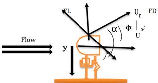
The equation of motion of the oscillator, which is driven translational galloping, is given as [2].

The Sinusoidal force, drag and lift forces can be written as [11]: 

Where C_L and C_D are the lift and drag coefficient curves,  the density of (flowing) medium and d effective area of the length cross section of the D- section. Now, The Sinusoidal force can be rewritten by substituting (13) and (14) in (12). 

Where y = 0. In this case, the motion might be small. When the motion is small, can be considered equal to zero as figure 2 shows value. Why α equalled to zero, it can be explained by as a result of the special Phenomena is called static divergence. This phenomenon's explanation is that no oscillation occurs but the model experiences a pure heave or pitch motion which is interpreted as a loss of vertical stiffness Therefore, the Taylor expansion can be defined below. Where the m is the mass per unit length, damping and stiffness coefficients c, and k per unit length [11].

For small  but  should be less than one, can be written as below [11] [12]. In this case, the non-dimensional parameters should be written.

Substituting   in equation (15).

After proofing all the parameters for each unknown symbol, now, they should be substituted in the main equation of motion:

Whereas the total damping and the damping ration can be written as [3].

Substituting (23) in (20). The translational galloping equation of motion of D- Section can be defined as:

This above equation (2.3.13) is equation of motion which can be used to simulate some geometrical shapes like D-section or square- section. The D-section, where the body was subjected to various flow velocities in varying angles (0, 45, 90, 135, 180, and then 0)⁰, can be similar to a semi-circle or a square of cross section area in some cases. Therefore, one of paper’s contribution is that the equation of motion for this model can be used to both of D-section and square section. This situation can be helpful for people who try to develop one degree of freedom aero dynamic galloping.

In this work, when the body was subjected to flow velocities in angle 0⁰, the body was seemed like a semi-circle of the cross-section area. Whereas when the body was subjected to flow velocities in angle 180⁰, the body seemed like a square of cross section area. Therefore, this equation could be worthwhile for some geometrical shapes. However, each shape has different geometrical properties, so the simulation should be different.

3. The Experimental Apparatus

As the below pictures are shown that the system are consisted of the one degree of freedom aero dynamic galloping with viscous damping coefficient C_s and spring stiffness K_s. The model was installed on a pace of steel by screw to prevent any doubt of the body movement by external force. The system was completely installed by using some available devices and equipment in the lab. The equipment and devices, which were used for experimenting the flow velocities effect on the mass, have many features and characteristics that will be given below in more detailed:

1. The fan has big two wings and made from steel, it is so-called a wind tunnel.

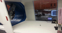
2. A big wood room was directly connected with the fan, it was built from both sides with glass walls to help the flow of the air moved smoothly in one direction while the many small holes were made on the back wall to prevent any pressure result of the air inside the chamber that could cause stillness case in movement of the body, so the air should be passed through back screen.

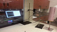
3. Two stands put inside a room, one carries a flowmeter and another one holds a laser sensor.

4. The flowmeter was used to measure flow velocities, it was consisted from two parts. the first part, which was sat up inside the chamber, measured the dynamical movements which was coming from the wind tunnel while the second part, which was connected with the first part by wire, was electronic device used to record actual flow velocity.

5. A laser sensor with specifications (intelligent –LIL, Laser sensor, Keyence/ IL 030)

6. Data Acquisition set up.

7. Wires connect.

8. Digital Sensor gauge (Keyence, IL Series, IL -1000), (Brown 10-30 VDC= 180 W max, Class2 or Lps).

9. The Computer has LabVIEW app 2012 SP1 (32-bit).

10. The resistance was used to increase and decrease fan speed (AC Power Supply).

4. The Experimental Procedures

The experimental procedures for D- Section model were finished after the system was built from devices above. The first step of experiment of the D- section was to increase gradually flow-velocity with keeping the angle of model equal to zero.

In this step, the flowmeter was shown flow velocities value which caused in the model oscillation, the excitation of body was transferred to a computer by a sensitive laser sensor, which was installed close and on the smooth area in the model. The excitation signal was recorded on the computer to draw figures between the time on X- axis and the displacement in range -5, 5 on the Y- axis. In this case, the excitation figures of the body was drawn for each flow velocity. Hence these figures were used to plot response curves for various flow velocities vs. amplitude. The procedure was repeated many times with each angle for the D-Section installed in front of the wind tunnel. The model was turned around itself gradually until it was reached 180⁰. The angles (0, 45, 90, 135, 180, and then 0)⁰ were done with various flow velocities. Therefore, the experimental procedures were finished with varying angles.

5. The Experimental Results and Discussion

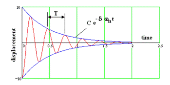
The design of a building or industrial tools for big cross- section areas need the expectation of the flow induced vibration an elastic - structure. Such expectations are the goal of programs like SHEAR7 (Van diver et al., 2011) that has been used in industry since 1990s. In this work, the D- section was designed with a big cross section area, and it was subjected to various flow velocities to known  cross-flow vibration in describe flow velocity and frequency. Hence begun the need to find a natural frequency to the body oscillation, the process, which was used to find a natural frequency, was completed by plotting a pluck test for amplitude vs. Time as shown in the figure 5.

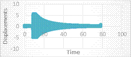
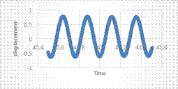
From (figure 5), it can be taken a part of the steady state amplitude (figure 6) to find a natural frequency as shown in this calculations. 
T1 = 40.887 Sec,       T2 = 41.124 Sec.
T= T2 – T1                          T= 0.237 Sec.
X1= 0.762879 mm    X2= 0.754131 mm
Where T represents a time, X represents an amplitude.
For successive amplitudes m = 1

 = Factor reduction amplitude = 0.011533
  Square both sides


 = 0.00000337        = 0.00183

Table 2. Showing the actual geometrical properties of model.

The mass	The stiffness	The natural frequency	The damping ratio
0.7438032 Kg	1144.8641 N/m	4.219 red/Sec	0.00183

From these steps above, it can be seen that the D - structure was oscillating in the natural frequency 4.219 rad/sec, and ζ = 0.00183. Therefore, it would be good enough to see a body excitation with range -5, 5 on the computer, and also it can be helpful to manipulate in the weight of the model mass. Hence the body was developed to one degree of freedom which the weight of the body mass is 0.7438032 Kg, and stiffness 1144.8641 N / m.  The table 3 shows the values of amplitude, which are in the positive side of displacement versus time figures, divided by D.

Table 3. Shown the experimental data for all the velocities and the amplitudes before and after the amplitude was divided by the section diameter.

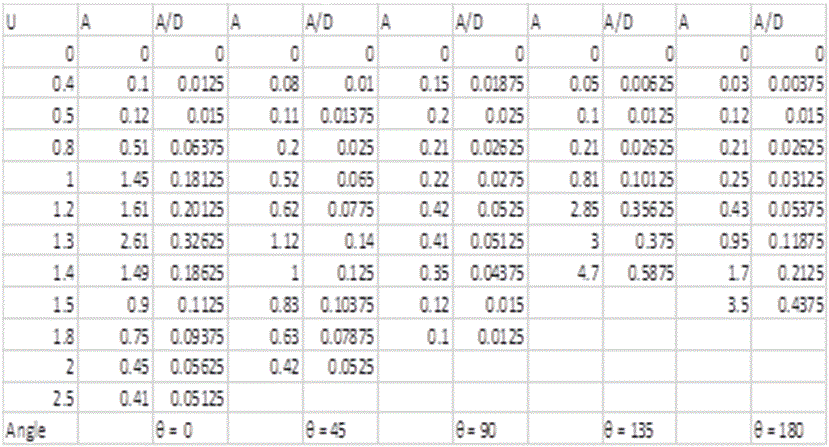
The excitation boundary (amplitude “A”) is found by successively solving the system for an increasing wind speed V or a decreasing , respectively, until an Eigenvalue enters the positive real quadrant. Here, the excitation occurs before static divergence. However, if the table 3 shows the square values of amplitude A², which are in the positive side of displacement versus time figures, divided by D, A²/D means that as an eigenvalue with a positive real part occurs in higher level than in A/D at the same velocity, the system is unstable and prone to flutter. In addition, amplitude value “A” represents a steady state amplitude for each figure of an amplitude vs. Time which repeated it for each flow velocity "this process is as same as process shown in figure 5, 6, but it was repeated many time for each a flow velocity". Amplitude vs. Time is plotted on the computer by a signal of a pluck test.

The experiments were done in many expectations on the D- structure. For example, Altering of flow velocities, and Altering the body case in various attack angles in front of the fan, consequently, the results were given many the periodic response figures which were drawn on the computer (as the appendix is shown). These figures were used to plot response curves between A/D versus velocities after collecting steady state amplitude data from each a periodic response figure as shown in the table 3. After having all data, the empirical values of experiment of the body aero dynamic galloping were represented in several response curves between flow velocities and the amplitudes and in the various attack angles, so the analysis of the D- section excitation are explained based on the body case in this experiment. The flow velocity increase of air rises of the body oscillation, this could be normally understood. However, this work was truly discovered a real behaviour for the body vibration when the body was made various responses of oscillation at the same angle, the non-symmetric body, which was subjected to various velocities and in various attack angles, make the amplitude  increased with velocities increase in the begun, but at the certain flow velocities, there was some change happened, the amplitude was taken linear stable behaviour that is called a lock - in region as shown in the below figures. The reason for lock - in region is a vortex - induced oscillation accompanied by the frequency synchronization with the D- section frequency by vibration, also result of self - excited. The lock - in region phenomenon is clearly examined by study (Sarpkaya 2004, Bearman 1984) [14] [15].

From above a brief statement of the lock - in region phenomenon, the figures will be clearer if they are discussed individually.

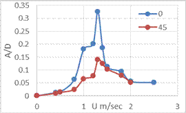
At the 0⁰ angle, which is considered the standard attack angle of D- Section and where the body was installed in front of the wind tunnel with a semi-circle of cross section area, will be compared to all attack angles of D- Section (45, 90, 135, and 180)⁰. In the standard case for body which is at the 0⁰ attack angle, the air flow passed, so the air pressure, which may be symmetrical amount on both sides, generated the many forces in perpendicular direction on the cross- section area of the D- section, these forces could vibrate the body regularly. Hence the flow velocity increase was caused in amplitude increase of body oscillation (figure 7). However, due to semi-circle of cross section area of the body, the galloping mechanism was happened by asymmetric aerodynamics of conductor.  After the asymmetric aerodynamics of conductor, the flow velocity increase of air was working to decrease sudden the body oscillation due to fs was close to fn. Hence, this was a unique phenomenon that has been happened which was caused by the shedding frequency is called vortex lock-in. Whereas when the attack angle changed to 450, the same phenomena was repeated as shown in the curve (figure 7), but it was happen at small periodic excitations. The reason for that phenomena was result of the air pressure was not asymmetric on the both sides of the body, so flow velocity of air faced some of the barriers which represents with the area of quarter circle on one side. These barriers raised of drag force.

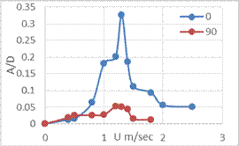
At the attack angle change to 90⁰ (figure 8), the flow velocity increase of air was accompanied a small increase of amplitude due to the differences between a cross section area on both sides, but thanks to the flow velocity of air increase, the body movement was taken a stable oscillation for a while due to the lift force was close to the drag force. This phenomenon is called lock - in region which related with other variables like frequency. Whereas the flow velocity increase of air was accompanied an increase of amplitude value due to a smooth area on one side, this increase was accompanied the galloping mechanism which happened at small amplitude and high velocity compared to the attack angle 0⁰.

At the attack angle change to 135⁰ (figure 9), the behaviour could be more different than other angles.  The amplitude versus velocity curve at 135⁰ angle seemed normal in the begun (figure 9), even though the body has non- symmetrical cross- section of area, the aerodynamic instability caused in the amplitude increase directly proportional with flow increase.

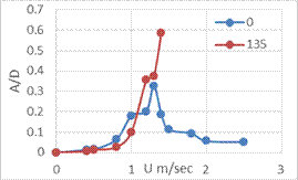
At the certain velocity, the amplitude was gone up and this change in behaviour was moved on until the model got in lock- in region. After the lock- in region that velocity increase was working on the amplitude increase. This behaviour caused result of pressure force of air in perpendicular direction on the side cross- section of the body area which also caused in changing vortex shedding.

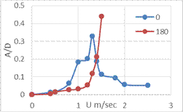
At the attack angle change to 180⁰ (figure 10), the vortex shedding resonance could be happened at high flow velocity, thus the turbulence might be caused upstream of the body.

Whereas, the small value of the turbulence wind tunnel has turbulence value no more than tenths of a percentage of the free flow velocity. The figure is shown that the amplitude is suddenly increased after flow velocity 1 m/ Sec which is called unstable flow.

Finally, this work can be concisely described by making a comparison between the flow -induced vibration on a D-section and a square section.  The results obtained which represent as curves are for the flow around a single degree of freedom SDOF "D-section” show at typical response of vortex-induced vibrations VIV at low Reynolds numbers and low mass ratio.  Figure 10 shows two curves included 1. “The body angle “0⁰” is that the body seems as a D-section in front of a wind tunnel 2. The body angle “180⁰” is that the body seems as a square section in front of a wind tunnel. In these two cases, the behaviour of these curves are totally different between each other as a result of differences of their cross sectional areas, cross sectional areas can cause to absence some phenomenon in one of the these models behaviours compared to the second model behaviour. For example, vortex lock-in, which results by the shedding frequency, does not be clearly shown or totally disappears from behaviour of square- section. In addition,  in the square- section, the vortex shedding resonance happens at high flow velocity which cannot happen to  D-section, thus the turbulence might be caused upstream of the body. 

6. Conclusion

The main objective of the analysis presented in the paper is to predict of the effect of various flow velocities on geometrical shapes and specifically on D- Section. Therefore, the attack angle change could have a good effect to decrease the vibration caused by the flow. The D- section  is developed from one degree of freedom aero dynamic galloping, and The D- section is a non- symmetric body with the actual geometrical properties are m= 0.7438032 Kg, K= 1144.8641 N/m, the natural frequency 4.219 rad/sec, and ζ = 0.00183, and  the equation of motion which were mentioned in this paper. The prospective suggestions for future to develop this model is to design D- section with small two wings on the both sides of the model with width no more than a quarter of the radius of the model. For example, if the diameter of the model D = 8 cm, the wings measurement width are 1 cm. these wings should be filled with holes to avoid the vortex shedding and the galloping. In conclusion, D- section is used to the design of a building or industrial tools for the big cross- section areas need the expectation of the flow induced vibration an elastic - structure.

References

[1] D. Brika and A. Laneville, "The flow interaction between a stationary cylinder and a downstream flexible cylinder," Journal of Fluids and Structures, vol. 13, no. 5, pp. 579-606, 1999. View Article
[2] A.H.P. van der Burgh and Hartono, "Rain-wind-induced vibrations of a simple oscillator," International Journal of Non-Linear Mechanics, vol. 39, no. 1, pp. 93-100, 2003. View Article
[3] J. K. Vandiver, "Damping Parameters for flow-induced vibration," Journal of Fluids and Structures, vol. 35, p. 105-119, 2012. View Article
[4] R. Govardhan and C. H. K. Williamson, "Defining the "modified Griffin plot" in vortex-induced vibration: revealing the effect of Reynolds number using controlled damping," Journal of Fluid Mechanics, vol. 561, pp. 147-180, 2006. View Article
[5] A. Khalak and C. H. K. Williamson, "Motions, forces and mode transitions in vortex-induced vibrations at low mass-damping," Journal of Fluids and Structures, vol. 13, no. 7-8, pp. 813-851, 1999. View Article
[6] J. T. Klamo, A. Leonard and A. Roshko, "On the maximum amplitude for a freely vibrating cylinder in cross-flow," Journal of Fluids and Structures, vol. 21, no. 4, pp. 429-434, 2005. View Article
[7] E. Finot, A. Passian and T. Thundat, "Measurement of Mechanical Properties of Cantilever Shaped Materials," Sensors, vol. 8, no. 5, pp. 3497-3541, 2008. View Article
[8] "Semicircle: Definition, Perimeter & Area Formulas," SBA Math, [Online]. Available: http://study.com/academy/lesson/semicircle-definition-perimeter-area-formulas.html.
[9] S. K. Mondal, Strength of Materials: Notes for IES, GATE & PSUs, 2013, pp. 1-431. View Article
[10] T. T. William and M. D. Dahleh, Theory of Vibration with Applications, Upper Saddle River: Pearson Education (US), 1997. View Article
[11] M. S. Zabarjad, "Determination of Galloping for Non-Circular Cross-Section Cylinders," PolyPublie - Polytechnique Montréal, Montréal, 2014. View Article
[12] R. D. Blevins, "Flow induced vibration of bluff structures," CaltechTHESIS, California, 1974. View Article
[13] Vandiver et al., "Fluid-Structure Interactions Using Analysis, Computations, and Experiments," in SHEAR7 User's Guide MIT, Dordrecht, Kluwer Academic Publishers, 2011, pp. 1-6.
[14] T. A. Sarpkaya, "A critical review of the intrinsic nature of vortex-induced vibrations," Journal of Fluids and Structures, vol. 19, no. 4, p. 389-447, 2004. View Article
[15] P. W. Bearman, "Vortex Shedding from Oscillating Bluff Bodies," Annual Review of Fluid Mechanics, vol. 16, pp. 195-222, 1984. View Article
Appendix
MATLAB CODE
time=[]; comment,
between brackets should be data.
amplitude=[];
figure;
plot(time,amplitude);
title('Amplitude vs. Time'); xaxis('Time');
yaxis('Amplitude');
grid on fs=300;
m=length(amplitude);
x=pow2(nextpow2(m));
y=fft(amplitude,x);
f=(0:x)*(fs/x);
p=y.*conj(y)/x;
figure; plot(f(1:value(x/2)),p(1:value(x/2)))
title( 'Power Spectrum'); xaxis('Frequency');
yaxis('Magnitude');
y=rms(amplitude); grid on