Journal of Fluid Flow, Heat and Mass Transfer (JFFHMT)
ISSN: 2368-6111

Volume 2 - Year 2015 - Pages 26-33
DOI: 10.11159/jffhmt.2015.004
Experimental Investigation on Pulsating Flow in a Bend
Masaru Sumida, Takuroh Senoo
Kindai University, Faculty of Engineering
1 Takaya Umenobe, Higashi-hiroshima, 739-2116 Japan
sumida@hiro.kindai.ac.jp
Abstract - An experimental investigation was conducted on a pulsating turbulent flow through a 90° bend with a circular cross section. The experiments were carried out under the conditions of Womersley number α=20, mean Reynolds number Reta=20000 and oscillatory Reynolds number Reos=10000 (flow rate ratio η=0.5). The time-dependent wall static pressure and axial and secondary flow velocities were measured at several longitudinal stations by laser Doppler velocimetry and the distributions are illustrated for representative phases. The distributions of the phase-averaged velocity are very different from those for a steady flow. Furthermore, they show complex changes along the tube axis.
Keywords: Pulsating Flow, Bend, Velocity Distribution, Secondary Flow, LDV.
© Copyright 2015 Authors - This is an Open Access article published under the Creative Commons Attribution License terms. Unrestricted use, distribution, and reproduction in any medium are permitted, provided the original work is properly cited.
Date Received: 2015-05-07
Date Accepted: 2015-11-06
Date Published: 2015-12-01
1. Introduction
Flows in both bends and curved pipes have been examined for a wide range of industrial uses, such as heat exchangers and elements in various piping systems, by many researchers in fluid mechanics. Most of the studies have mainly been concerned with steady flows [1]. In particular, the secondary flows generated in the cross sections of curved pipes and bends have attracted the interest of researchers. Recently, the interest in secondary flows has extended to the unsteady decay behavior in pipes downstream of bends [2, 3] in addition to the formation and transition processes. On the other hand, the research on unsteady flows started in the 1970s and has progressed rapidly [4-6]. However, researchers have focused on the flow of blood in arteries. Therefore, they limited their investigation to laminar flows with relatively low Reynolds numbers.
From an industrial viewpoint, turbulent unsteady flows are very important. However, there have been few works on such flows [7-11]. Sumida et al. [9] developed an approximate method for analyzing the pressure gradient in a fully developed pulsating turbulent flow in curved pipes. They presented useful expressions relating the governing parameters and the pressure gradient. Also, Sumida [10] proposed a method of obtaining pulsatile flow rates by measuring the pressure difference across the cross section of a 360° bend. On the other hand, Sohn et al. [11] measured velocity distributions for a 180° curved duct by laser Doppler velocimetry. There are many industrial piping systems with bends and elbows having a turn angle of 90°. Iguchi et al. [7] and Sano et al. [8] have investigated flows in such cases. In the former study [7], the pressure losses of 5/4 and 1/2B JIS screwed elbows fitted by the expansion of the joint were evaluated for pulsating flows. The latter study [8] considered the case where undeveloped flows with an almost uniform axial-velocity distribution and a small flow rate ratio were introduced into the bend. However, to understand the characteristics of a pulsating turbulent flow in a bend, it is first desirable to examine flows with a large flow rate ratio and a fully developed entry-flow condition in a smooth bend. No measurements have been reported for a fully developed pulsating turbulent flow entering the 90° bend of a pipe with a circular cross section, despite the many practical uses of such a pipe. Therefore, the understanding of the flow behavior in such bends is insufficient.
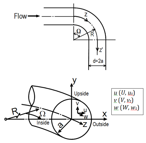
The pulsating turbulent flow in a 90° bend is governed by four nondimensional parameters: the Womersley number α, the mean Reynolds number Reta, the flow rate ratio η and the curvature radius ratio Rc. Here, the Womersley number is a frequency parameter and is defined as α=α(ω/ν)1/2, with α being the radius of the pipe, ω the angular frequency of pulsation and n, the kinematic viscosity of the fluid. The mean Reynolds number is expressed as Reta=Wa,ta d/ν, in which Wa,ta is the time-mean value of the cross-sectional averaged velocity Wa and d(=2α) is the inside diameter of the pipe. η=Wa,os/Wa,ta is the ratio of the amplitude value Wa,os of Wa to Wa,ta. Finally, Rc is given by Rc=R/α, with R being the curvature radius of the bend axis. However, it is difficult to treat the flow problem including all these parameters for the current situation.
In this study, we consider the problem of a pulsating turbulent flow through a 90° bend with Rc=4. Furthermore, we investigate the flow with α=20, Reta=20000 and η=0.5 as representative flow conditions to extract the flow features. That is, measurements were made for the axial and secondary flow velocities and the wall static pressure by laser Doppler velocimetry (LDV) and using a diffusive semiconductor differential-pressure transducer, respectively. We discuss the periodic changes in their phase-averaged distributions along the bend axis.
2. Experimental Apparatus and Measurement Method
A schematic diagram of the experimental apparatus employed in this study and the coordinate system are shown in Figs. 1 and 2, respectively. In Fig. 2, the additional coordinate z’ is introduced to represent the distance measured along the pipe axis from the bend exit for convenience. The apparatus is composed of a pulsating flow generator, a test bend, and velocity and pressure measurement devices. The working fluid was water at a constant temperature of 20°C. The test bend was made from accurately machined transparent acrylic plates. The inside diameter was d(=2α)=22.0 mm and the curvature radius was R=44 mm, giving a curvature radius ratio Rc(=R/α) of 4. Upstream and downstream straight sections of 70d and 28d lengths, respectively, were connected to the bend. The volume-cycle pulsating flow was generated by superimposing an oscillating flow driven by a piston installed in a scotch yoke mechanism on a steady flow supplied by a pump. Thus, the instantaneous axial velocity averaged over the cross section, Wa, can be expressed in the form

Here, Θ(=wt) is the phase angle, with w and t being the angular frequency and time, respectively. Moreover, the subscripts ta and os indicate time-mean and amplitude values, respectively.
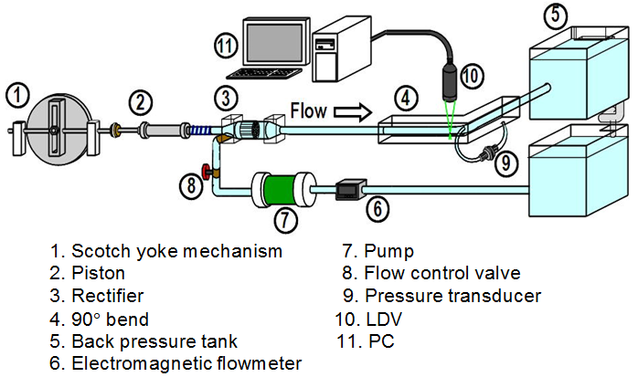
In the experiment, the instantaneous velocities, w and u, in the axial and outward directions, respectively, and also the instantaneous wall static pressure p were obtained. The wall static pressure was measured by a diffusive semiconductor differential-pressure trans-ducer (JTEKT Corp., DD102A-0.1F), which has a frequency characteristic of about 600 Hz in air. Measuring taps of 0.6 mm diameter were drilled into the upside, inside and outside walls of the test bend. Moreover, a laser Doppler velocimetry (Kanomax, Ser. 8835) was used for the velocity measurement. The LDV system was a two-component type with a 3 W Ar ion laser source and was operated in backscattering mode. In the present experiment, we used green laser light with a wavelength of 514.5 nm and a lens with a focal distance of 192 mm with a laser-beam cross angle of 9.53° in air. In the LDV measurement, the test bend was placed in a water bath to reduce the effect of the refraction of the conduit wall on the laser beam optics, as shown in Fig. 1. The pressure and velocity measurements were performed at 11 streamwise stations, including five stations in the bend, between z=-8d in the upstream pipe and z’=10d in the downstream pipe. The velocity data at the stations were obtained on the x- and y-axes, except for the station at z/d=-2. Moreover, the velocity was measured at 20-25 points on each axis.
The outputs from the amplifier of the pressure transducer and from the signal processor of the laser Doppler velocimetry were sampled using a personal computer synchronously with a time-marker signal that indicates the position of the piston. The data at each measuring point were taken for 200 to 300 pulsation cycles with 360 to 500 samplings per cycle. For a periodically unsteady turbulent flow, any instantaneous quantity, such as the axial velocity w in the pulsation cycle, can be written as

Here, W is the phase-averaged velocity and wt is the fluctuating velocity, in which the subscript t indicates fluctuating quantity. The turbulence intensity w’ was obtained as the square root of the ensemble phase average of wt2. Similar statistical analysis was also performed for the pressure. It was confirmed beforehand that averaging over 200 cycles has no effect on the values obtained, although the number of pulsation cycles used for the ensemble average was varied according to the measured section and radial position.
In the LDV measurement, there were errors in the cross angle of the laser beam and the positioning of the measured volume owing to the curvature effect of the test bend. The former resulted in an error of 0.6% in the velocity. The errors in the local velocity caused by the positioning error and the accuracy of the traversing system were estimated to be less than 3%. Therefore, the measurement error was estimated to be less than 4%. Moreover, the errors occurring in obtaining the turbulence statistics were combined with the above measurement errors. As a result, the combined total error of the present data was estimated to be 5% for the phase-averaged velocity and pressure and 8% for the turbulence intensity.
The experiments were performed under the conditions of α=20, Reta =20000 and η=0.5, which were selected with reference to previous works [7-12] on pulsating turbulent flows in pipes and a duct.
3. Results and Discussion
To verify that the flow entering the bend is the desired flow, preliminary measurements were conducted for the axial velocity at z/d=-2 in the upstream pipe. The time-dependent flow rate Θ was calculated by integrating the velocities measured at 144 positions over the cross section. The result is shown in Fig. 3, where the solid line denotes the prescribed sinusoidal flow rate provided by the pulsating flow generator. The calculated and prescribed flow rates are in good agreement. This confirms that the prescribed flow is realized in the test bend and also that a sinusoidal flow rate that can be expressed in the form of Eq. 1 is obtained.
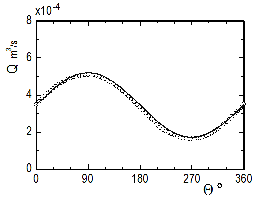
(α=20, Reta=20000, η=0.5)
3. 1. Changes in Wall Static Pressure with Time
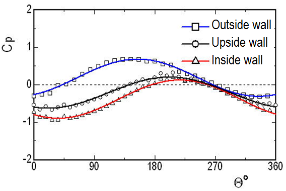
The phase-averaged wall static pressure P is expressed in the form of the pressure coefficient Cp, which is defined as

Here, Pref is the pressure acting on the upside wall at the station with z/d=-2 in the upstream pipe and ρ is the density of the fluid.
In this study, we examine the phase-averaged value of the pressure. Figure 4 shows the periodic variation of the difference between the pressure at z/d=-2 and that at the bend exit (Ω=90°). Cp at the outside wall is larger than that at the inside wall throughout the period. However, the pressure at the outside wall has an adverse gradient for most of the period (Θ≈40-270°), i.e., from the middle of the accelerative phase to the phase with the minimum flow rate. By contrast, the pressure at the inside wall exhibits a favorable gradient except for when Θ≈180-260°. The pressure differences in the cross section, for example, the differential pressure across the outside and inside of the bend, are large and small in the phases with a large flow rate (Θ»0-180°) and a small flow rate (Θ≈180-360°), respectively. Moreover, the phase difference between the variation of Cp at the inside wall and that at the outside wall is about 63°. Thus, the change in pressure with time in the bend is considerably dependent on the location in the cross section.
3. 2. Phase-averaged Velocity
For a pulsating turbulent flow through a bend, the mixing action by turbulence and the variation of the secondary flow with time affect the velocity distri-butions significantly. Therefore, the characteristics of the velocity distributions are different from those in laminar flows [4-6], which have been examined up to now. It is forecast that the velocities in the pulsating turbulent flow will have very complex distributions. In this paper, we investigate the phase-averaged velocities of W and U. We first give an outline of the flow features by focusing on the axial velocity W on the bend axis.
Figure 5 shows waveforms of W at the radial positions of x/α=0 and ±0.8. The phase-averaged axial velocity W changes almost sinusoidally with time. However, the amplitude of W on the pipe axis is reduced in the bend. The phase lead of W relative to the variation of the flow rate becomes large and reaches about 30° at the bend exit (Ω=90°). On the other hand, in the upstream pipe, the periodic change in the axial velocity W near the pipe wall slightly precedes the variation of the flow rate owing to the viscous force, as shown in Fig. 5a (x/α=±0.8). In contrast, in the central part of the cross section, W exhibits a phase lag owing to the unsteady inertia force (Fig. 5a, x/α=0). However, in the bend, the amplitude of W becomes large near the outside wall, whereas near the inside wall, it is reduced, and W at Ω=90° also changes with a phase lag. Thus, in the bend, the variation of the axial velocity on the pipe axis advances. The difference between the velocity amplitudes near the inside wall and outside wall becomes large. Therefore, unsteadiness is exhibited, with actions of the centrifugal and viscous forces, in the flow in a complicated manner.
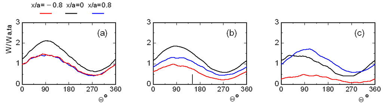
(a) z/d=-2, (b) Ω=60°, (c) Ω=90°.
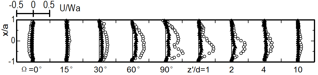
Figures 6 and 7 show the distributions of the phase-averaged velocities, W and U, on the x-axis, respectively. In the figures, the velocities are normalized by the time-mean value of the cross sectional average velocity Wa,ta. The profiles are illustrated for representative phases in a pulsation cycle. For comparison, the results for the steady flow at the same Reynolds number Reta are also presented in Figs. 8 and 9.
In the straight pipe upstream from the bend (z/d=-2), the periodic change in the axial velocity W with time advances slightly near the pipe wall from the variation of the flow rate Q shown in Fig. 3, whereas it is delayed slightly in the central part of the cross section. This is recognized by comparing the W distribution at Θ=0° with that at Θ=180° at the station with z/d=-2 in Fig. 6. Nevertheless, on the whole, the velocity at each phase shows an axisymmetric profile similar to that of
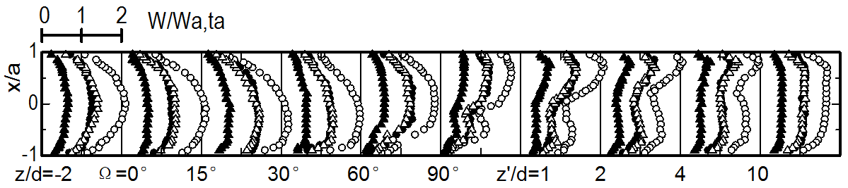
⚫: Θ=0°, ⚪: Θ=90°, △: Θ=180°>, ▲: Θ=270°.
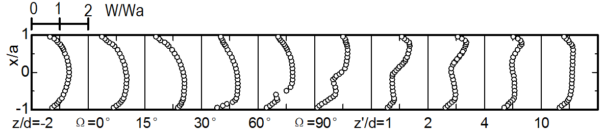
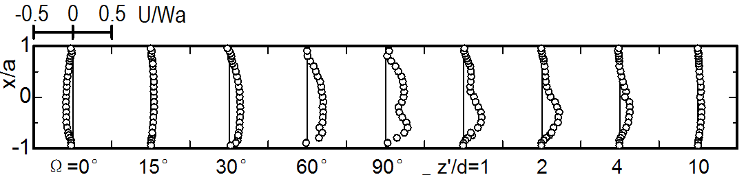
the steady flow. At z/d=-1, near the bend entrance, fluid with higher axial velocity in the central part of the cross section begins to move toward the inside wall in the latter half of the accelerative phase (Θ=0-90°) since the pressure rises on the outside wall. Immediately behind the bend entrance, Ω=0-30°, the acceleration of the fluid becomes largest in the inner region of the bend. Consequently, the position of the maximum axial velocity is biased towards the inside wall when the flow rate is large. The bias toward the inside wall at Ω=15-30° becomes large in comparison with that for the steady flow shown in Fig. 8 as the flow rate increases. At this time (Θ=90°), the secondary flow on the x-axis of the bend entrance (Ω=0°) has a negative velocity with a value approximately one-tenth of the maximum Wa. On the other hand, the fluid with a higher speed in the central and outer regions of the cross section is subjected to a strong centrifugal force. This forces the direction of the secondary motion to change towards the outside wall (Ω=15°). Consequently, the outward velocity U at Ω=30° becomes approximately 50% higher than that in the steady flow at the same cross-sectional average velocity Wa,ta. Moreover, U still increases compared with that in the steady flow as the fluid flows around the bend. Further downstream (Ω=60°), the region with a higher axial velocity begins to shift toward the outside wall. As a result, the axial velocity near the inside wall decreases rapidly, and consequently its variation becomes small.
At the bend exit (Ω=90°), fluid with a higher speed flows into the inside wall region along the upside and downside walls. The fluid in the central part of the cross section, in contrast, is swept toward the outside wall by the strong secondary flow. Accordingly, the axial velocity on the x-axis has a distribution with two maxima near the inside and outside walls, while its distribution on the y-axis has a depression in the central part. On the other hand, the secondary flow velocity is high from the latter half of the accelerative phase to the first half of the decelerative phase (Θ=60-180°). During these phases, the U profile changes into a shape with two maxima, similarly to the distribution of W. In particular, the outward velocity U is intensified compared with that in the steady flow in the inner part of the cross section.
In the straight pipe downstream from the bend exit, no centrifugal force acts on the fluid. Nevertheless, owing to the increased pressure on the inside wall, the outward velocity U significantly increases to as high as 50% of Wa,ta (z'/d=0-2). Therefore, the depression in the W distribution becomes notable at z'/d=1 and the degree of depression is greater than that in the steady flow. Further downstream, however, the axial velocity increases in the inner region from the center of the cross section. The distribution of W gradually becomes flat in the cross section at z'/d=4-10. However, the flattening of the W distribution is retarded when the flow rate is large. At z'/d=10, the W distribution has not yet recovered to that observed in the upstream straight pipe.
3. 3. Deviation of Axial Flow and Intensity of Secondary Flow
As stated in section 3.2, a pulsating turbulent flow through a bend exhibits very complicated behavior. In particular, the distribution of W has a difference in shape in the inner and outer parts of the cross section and also in the streamwise direction of Ω and z’. Thus, we examine the effect of the local axial velocity amplitude Wos on the W distribution. Here, the phase-averaged velocity W is decomposed into the time-mean component Wta and sinusoidally varying components Wos,i. That is, we express the measured W by a Fourier series with respect to time as follows:

Here, Φi is the phase difference of the ith varying component Wos,i from the flow rate given by Eq. 1. In this study, we consider the first component Wos,1 and omit the suffix 1 for convenience, i.e.,

Then, we define the deviation of the axial velocity amplitude using the Wos distribution on the x-axis and introduce the following quantity:
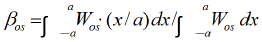
where βos denotes the bias of the Wos distribution on the x-axis.
Figure 10 shows the deviation of Wos. In Fig. 10, values of βst obtained from the W distribution of the steady flow shown in Fig. 8 are also shown for reference. The axial velocity amplitude Wos starts to become biased toward the inside wall in the straight pipe close to the bend entrance. The bias toward the inside wall is greatest at Ω=15°. Afterwards, it rapidly reverses direction toward the outside wall, and βos immediately behind the bend exit has a maximum value of about 0.17. In the downstream straight pipe, the bias toward the outside wall persists until a considerable distance downstream, although βos rapidly becomes small. Comparing βos with βst, the change in βos along the pipe axis is considerably smaller than that in βst.
⚪: βos, ⚫: βst for steady flow at Re=20000.
⚪: Θ=90°, △: Θ=270°, ⚫: Steady flow (Re=20000).
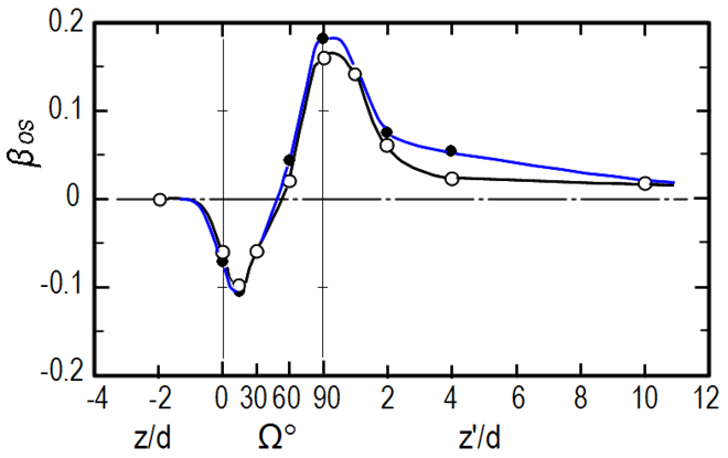
Finally, we investigate the intensity of the secondary flow, which we evaluate using the absolute values of the secondary flow velocities in the outward direction, U, on the x- and y-axes as follows:
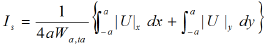
Here, the subscripts x and y indicate the x- and y-axes, respectively. The intensity of the secondary flow is shown in Fig. 11. The secondary flow intensifies from the vicinity of the bend entrance. At the maximum flow rate (Θ=90°), its strength Is takes a maximum value at the bend exit, while Is at the minimum flow rate (Θ=270°) has a maximum at Ω=60°. Downstream, the secondary flow rapidly becomes weak at the two phases. The time-averaged value of Is is large immediately behind the bend exit compared with that in the steady flow at the same Reynolds number Reta. At z’/d=10 in the downstream pipe, the secondary flow still has a speed of 2-4% of Wa,ta.
4. Conclusions
An experimental investigation has been performed on a pulsating turbulent flow through a 90° bend with a curvature radius ratio of Rc=4. The flow velocity was examined by LDV for the conditions of α=20, Reta=20000 and η=0.5. The findings of this study are summarized as follows:
- The flow exhibits very complicated characteristics significantly different from those of a steady flow, and the velocity and pressure distributions change in an intricate manner with the phase Θ and also in the streamwise direction Ω and z’.
- The difference in pressure between the entrance and exit of the bend is larger on the outside wall than that on the inside wall through a period.
- The axial velocity W near the bend entrance is higher near the inside wall when the flow rate is large, while W near the bend exit has a depression in its distribution. And also, the changes in the Wos distribution along the bend axis strongly affect the time-dependent distribution of W. The bias of the axial velocity amplitude is smaller than that in the steady flow.
- The secondary flow is strongest near the bend exit and then gradually attenuates. Nevertheless, it does not disappear even at z’/d=10, at which the flow has still not recovered to the straight pipe flow.
Acknowledgements
The authors thank Mr. J. Yamamoto, who helped set up the experimental apparatus during his postgraduate research at Kindai University. Furthermore, this work was supported in part by MEXT-Supported Program for the Strategic Research Foundation at Private Universities (Grant No. S0901045).
References
[1] H. Sugiyama, “Flow in curved pipes,” Nagare, vol. 22, no. 1, pp. 41-50, 2003. View Article
[2] J. Sakakibara and N. Machida, “Measurement of turbulent flow upstream and downstream of a circular pipe bend,” Physics of Fluids, vol. 24, 041702, 2012. View Article
[3] F. Rütten, W. Schöder and M. Meike, “Large-eddy simulation of low frequency oscillations of the Dean vortices in turbulent pipe bend flows,” Physics of Fluids, vol. 17, 035107, 2005. View Article
[4] M. Jarrahi, C. Castelain and H. Peerhossaini, “Secondary flow patterns and mixing in laminar pulsating flow through a curved pipe,” Experiments in Fluids, vol. 50, pp. 1539-1558, 2011. View Article
[5] M. Sumida, “Pulsatile entrance flow in curved pipes: effect of various parameters,” Experiments in Fluids, vol. 43, pp. 949-958, 2007. View Article
[6] B. Timité, C. Castelain and H. Peerhossaini, “Pulsatile viscous flow in a curved pipe: Effects of pulsation on the development of secondary flow,” International Journal of Heat and Fluid Flow, vol. 31, no. 5, pp. 879-896, 2010. View Article
[7] M. Iguchi, M. Ohmi and H. Nakajima, “Loss coefficient of screw elbows in pulsatile flow," Transactions of the Japan Society of Mechanical Engineers (Series B), vol. 50, no. 452, pp. 943-950, 1984. View Article
[8] K. Sano, K. Kikuyama, K. Koike and T. Oisi, “Pulsatile turbulent flow in a 90° bend,” Transactions of the Japan Society of Mechanical Engineers (Series B), vol. 61, no. 585, pp. 1722-1729, 1995. View Article
[9] M. Sumida, K. Sudou and T. Takami, “Pulsating flow in curved pipes: 2nd Report, Experiments,” Bulletin of JSME, vol. 27, no. 234, pp. 2714-2721, 1984. View Article
[10] M. Sumida, “Obtaining pulsatile flow rate using a 360-degree bend,” Universal Journal of Mechanical Engineering, vol. 3, no. 3, pp. 63-70, 2015. View Article
[11] H. C. Sohn, H. N. Lee and G. M. Park, “A study of the flow characteristcs of developing turbulent pulsating flows in a curved duct,” Journal of Mechanical Science and Technology, vol. 21, pp. 2229-2236, 2007. View Article
[12] M. Ohmi and M. Iguchi, “Flow pattern and frictional losses in pulsating pipe flow: Part 3, General representation of turbulent flow pattern,” Transactions of the Japan Society of Mechanical Engineers (Series B), vol. 46, no. 404, pp. 636-643, 1980. View Article