Journal of Fluid Flow, Heat and Mass Transfer (JFFHMT)

ISSN: 2368-6111

Heat-Kernel Parametric Model of Heat Transfer Through Layered Materials Coupled to Heat Sinks

Edward Michaelchuck Jr.¹, Jesse Duncan ¹, Scott Ramsey ¹, Troy Mayo¹, Samuel Lambrakos¹

¹U.S. Naval Research Laboratory
4555 Overlook Ave SW, Washington, D.C. 20375
Edward.Michaelchuck@nrl.navy.mil; Jesse.Duncan@nrl.navy.mil;
Scott.Ramsey@nrl.navy.mil; Troy.Mayo@nrl.navy.mil;
Samuel.Lambrakos@nrl.navy.mil

Abstract - A parametric model of heat transfer through layered materials is presented. This model is formally based on the heat-kernel solution to the advection-diffusion equation, which is extended to include effects of multiple layers with varying thermal diffusivities, interface effects (e.g., large changes in thermal properties), contact resistance, and the effects of singular heat-sinks, represented by negative heat sources. This model provides parametric representations of temperature distributions within layered-material systems, which can be utilized for their design and optimization for layer-configuration, including heat-sink control of thermal transport. Results of prototype modelling of controlled heat transfer in layered-material systems are presented and validated, demonstrating general aspects of the parametric model for thermal analysis and simulation of heat-transfer control using layer configurations and embedded heat sinks.

Keywords: Heat Transfer model, multi-layer materials, heat sinks, heat source distributions, basis function expansion.

© Copyright 2024 Authors - This is an Open Access article published under the Creative Commons Attribution License terms Creative Commons Attribution License terms. Unrestricted use, distribution, and reproduction in any medium are permitted, provided the original work is properly cited.

Date Received: 2023-05-19
Date Revised: 2023-12-14
Date Accepted: 2024-03-13
Date Published: 2024-03-26

1. Introduction

The control of heat transfer through multilayer materials is significant for many applications, ranging from heat treatment of materials to thermal management of systems. Optimizing heat transfer through multilayer materials requires estimating the thermal response of layered composite materials. This can be achieved using parametric models that combine heat-transfer characteristics of a specified layered system and thermal material properties, enabling prediction of temperature fields. These models should be conveniently adaptable for estimating the thermal response of different types of layered materials. The present study presents a parametric model of heat transfer through a layered material system. The parametric model is motivated by welding processes [1], where work piece temperatures are controlled by material composition and thermal contact to base plates. The control of heat transfer through multilayer materials can also utilize heat sinks. The general physical character of heat sinks is that their thermal diffusivities are substantially greater than those of the work pieces whose temperature fields are to be controlled [2]. Accordingly, thermal coupling of heat sinks to adjacent layers can be represented parametrically by phenomenological negative heat sources [3].

Parametric modeling of temperature fields follows the approach of inverse analysis [4], i.e., inverse thermal analysis [5-10], which is for estimating optimal parameter values for a given system specification. The parameter values (e.g., effective thermal diffusivities) should be achievable for realistic system design. For complex material systems, the determination of material response functions is well posed in terms of inverse analysis. The multiscale character of layered materials poses an inverse analysis problem, which follows from the realization that layered-material thermal properties are not the same as those of bulk materials. In addition, for layered materials there is typically influence on thermal transport due to advection at bounding surfaces of the layered system. Accordingly, parametrization should be extended to include effective diffusivities, which are based formally on replacing the advection-diffusion operator with an effective-diffusion operator. Physically, advection is not expected to manifest as influencing thermal transport locally within a layered-material system, but rather as influencing thermal transport over the its entire length of the layered system. Accordingly, the phenomenological influence of advection, which is associated with ambient environments at surface boundaries of a layered-material system, again poses a problem of inverse thermal analysis for determination of effective diffusivities. Finally, heat transfer across interfaces of layers making up a layered material system can be effectively singular with respect to heat-transfer trend characteristics because of thermal contact resistance and possible large differences of thermal diffusivity. Accordingly, with respect to parametric modeling, an interface may be represented by a layer having singular characteristics with respect to heat transfer. Heat transfer through a characteristically singular layer from adjacent layers of material will depend on the characteristic thermal coupling of layer interfaces, which again is a complex material property, not known a priori, and thus appropriately posed for inverse thermal analysis.

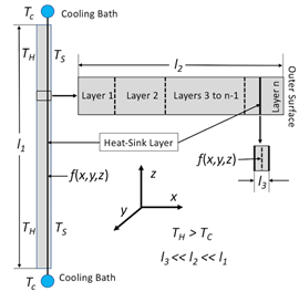
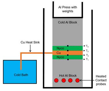
There exists different types of configurations for heat-sink coupling to a heated system. The parametric model considered here, for heat-sink coupling to a heated layered system, is described schematically in Figure 1, where coupling occurs at edges of the system. This configuration poses a specific problem with respect to inverse thermal analysis.

This study presents a parametric model for heat transfer through layered material systems, formally based on the heat kernel solution of the heat conduction equation [3], which includes effects of multiple layers with varying thermal diffusivities, interface effects (e.g., large changes in thermal properties), contact resistance, and the effects of singular heat-sinks (represented by negative heat sources). This model is structured for analysis of both steady state and time-dependent heat transfer in thin layered materials. In addition, this model is combined with another parametric model of heat-sink cooling, which is based on a specific approximation of the heat-kernel solution. Organization of subject areas presented are as follows. First, a parametric model of temperature fields for heat transfer through layer layered materials coupled to heat sinks is presented. Second, a formal mathematical analysis of the parametric model’s structure is presented, which provides physical interpretation of the parameters. Third, prototype simulations using the parametric model are described. Fourth, prototype inverse thermal analyses using the parametric model are presented. Finally, a discussion and conclusion are given..

2. Parametric Model

Presented in this section is a parametric model for heat transfer through a thin layered material heated at one surface, with transfer of heat to an ambient environment at the other surface by means of radiation and convection, with the possibility of heat-sink channel cooling, at steady state. For brevity of the document and to assist reader comprehension, a nomenclature section, Section 9, outlines the various variables present in the parametric model and associated equations.

The parametric model is based formal extensions and approximations of analytical solutions to the heat conduction equation [3], is given by

and

The quantities h_j, j = 1-N_j, are the interface contact-diffusivity parameters (analogous to contact conductance) whose units are 1/s, where locations of layer-layer interfaces are at x = x_j, and u(x) is the Heaviside unit step function. The source function f(x,y,z) is the 3D cooling field of the heat sink. The quantities τ_H,C₀, C₁, Q_x Q_y, and Q which are formally a delay time, a basis function scaling parameter, another basis function scaling parameter, and cooling fluxes, which specify heat flux at the heating boundary (parameter ) and strength of coupling of heat sink layer to a cooling bath (parameter ) to adjacent material layers (parameters ). Note that physically, for a given location (x,y,z), heat sink cooling is formally for all x, y and z. Our goal, however, is parametric modelling of heat transfer to the surface of the layered system, and therefore the region x > x_hs is of most interest. The function f(x,y,z) assumes a model representation that is, in principle, based on either physical assumptions, i.e., materials having known thermal properties or phenomenological parameters adjusted with respect to measurements. Specifically, the parametric model is defined in terms of adjustable parameters, τ_H, C₀, C₁, Q_x, Q_y, Q_z and ∆T_c which are determined in principle according to experimental measurements, i.e., inverse thermal analysis. Similarly, contact conductances, h_j, are adjustable parameters to be determined by measurements.

Referring to Eqs. (4) and (5), note that 0 < y-y_hs < L_y and 0 < z-z_hs < L_z The quantity L_z, which for present simulations has arbitrary units, is scaled according to the transverse length l₁ coupled to cooling bath as shown schematically in Figure 1. The quantity L_y (not considered here), together with L_z, represent two-dimensional coupling to a cooling bath.

Next, given a surface boundary at x = x_s, and letting T_S = T(x_s,y,z), defined by Eq. 1, for x > x_s,

The quantities h_c, e, s, and T_A are the convective heat-transfer coefficient, emissivity of the outer surface, Stefan-Boltzmann Constant (5.6704⸱10^-8 W⸱m^-2⸱K^-4) and the ambient temperature at the outer surface, respectively. Equations 1-6 define a parametric model for heat transfer through a layered material, from a hot body to a ambient environment external to the outer surface, with cooling due to an embedded heat sink.

3. Structure of the Parametric Model

This section examines the formal structure of the parametric model defined by Eqs. 1-6, which is for heat transfer through a thin layered material, heated at one surface, with transfer of heat to an ambient environment at the other surface by means of radiation and convection, with the possibility of heat-sink channel cooling. Heat transfer is assumed either at steady state or time dependent. Time dependency of heat transfer is assumed to be measured and represented parametrically by means of time-delay parameters according to inverse thermal analysis. This model is based on formal extensions of heat-kernel solution to the heat conduction equation [3], given by

Before proceeding with application of the model, there are key aspects of the type of layered system considered (see Figure 1), and its parametric-model representation Eqs. 1-6, that should be emphasized for model-parameter interpretation. These are:

1. The heat-kernel Eq. 8 is a convenient ansatz for parametric representation of time evolution, i.e., time-dependent heat transfer.
2. For both steady state and time-dependent heat transfer, the time-delay and cooling-flux parameters can be given physical interpretations.
3. The parametric model assumes that contact conductance between layers is dominant with respect to influencing heat transfer through the layered material system, relative to the influence of changes in thermal properties across an interface.
4. The parametric model Eqs. 1-6 is convenient for parameter adjustment with respect to boundary conditions on the system shown in Figure 1.
5. The thermal diffusivities can be either measured quantities (i.e., material properties), or themselves, adjustable phenomenological parameters.

The time-delay parameter may be interpreted by considering heat transfer to first order. Specifically, that the heat flux Q_H given by

for conductance k, integrated over interval (x, x_s) for a surface at T_H, gives

Next, Eq. 8 is reformulated to satisfy two boundary conditions, which are temperatures at the heating and outer surface boundaries of the layered material, and is thus

Next, assuming (x_s – x_o) is small, consistent with the condition of a thin layered material, it follows that

Comparing Eqs. 10 and 12,

It follows from Eq. 13 that the delay-time parameters, for “thin” layered materials (systems of our consideration) are inversely proportional to heat fluxes (or cooling fluxes), and accordingly, are physically consistent parameterizations of these fluxes. Finally, proceeding with analysis of Eq. 1, it can be seen that the source function f(x,y,z) is based on the approximation defined by Eqs. 12 and 13.

An important property of Eq. 1 is that, although it is structured for convenient encoding of time-dependence, based on the underlying heat-kernel ansatz, its mathematical property is that of tending toward piecewise linearity, i.e., formally Eq. 13. This is a manifestation of the underlying system, which is a “thin” layered material. This same property, tending to linearity, applies to Eqs. 3-5, representing heat-sink coupling. The ansatz for these equations is the approximation defined by Eq. 13, which is convenient inverse thermal analysis of heat-sink coupling to thin layered materials.

Temperature fields associated with both time-dependent and steady state heat transfer over an extended spatial region, as in welding processes, based on their spatio-temporal characteristics, may be modelled parametrically using linear combinations of weighted heat-kernel solutions, i.e., sums of heat-kernel puffs. This type of representation requires adjusting sets of weight coefficients according to evolving temperature fields extending over space as a function of time, and eventually achieving steady state. The property of Eq. 1, of tending to piecewise linearity, implies that a single heat-kernel puff is sufficient for parametric representation.

4. Prototype Simulations

This section presents simulations using the parametric model Eq. 1-6 of layer-configuration and heat-sink controlled thermal transport within a layered material system. The design of these simulations, using both physically realistic thermal properties and phenomenological adjustable parameters, was not to demonstrate optimal layer-configuration and heat-sink thermal control, but rather general characteristics of the parametric model for modelling and simulation of such control, as well as demonstrating feasibly of such control using multilayer and heat-sink materials. The simulations described in this section may also be interpreted as representing prototype inverse thermal analyses, which are a goal of parametric modelling, in addition to estimating thermal response of a system given parameter values.

The simulations presented in this section where programmed in MATLAB©. The prototype simulations selected an example material stack up with known material properties for the various layers. The simulations assume a specific performance with regards to heat transfer and heat sink performance. The simulations use a time independent, isothermal boundary condition for the hot boundary and a time dependent isothermal boundary condition for the cold boundary in the absence of a heat sink. The cold boundary condition is primarily for parameterization of the system; therefore, in the presence of a heat sink, the cold boundary condition is not enforced – only the hot boundary condition is enforced.

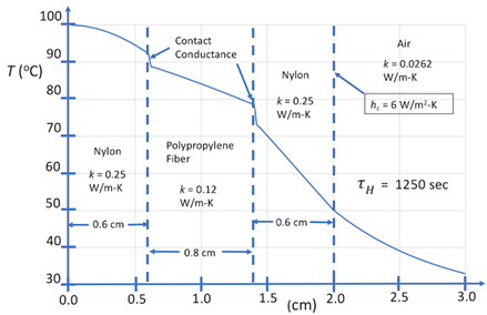
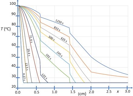
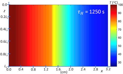
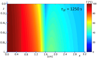
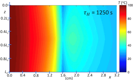
Our first prototype simulations are of heat transfer from a hot body at 100^oC through a layered system, using the parametric model defined by Eqs. 1-7, which are shown in Figures 2 and 3. These simulations assume contact conductance between layers, represented by equivalent contact diffusivities, which have been determined by inverse thermal analysis. The temperature fields shown in Figures 2 and 3 are modified in computational experiments that follow. Shown in Figure 2 is the temperature field of the layered system at steady state. Shown in Figure 3 is the time-dependent temperature field for evolution of this system to steady state. Referring to Figure 4, the model system considered here, neglecting y-dependence of heat-sink cooling represented by Eq. 3, is two dimensional and associated with four boundary conditions, which are specified at the heated and outer-surface boundaries, and at the boundaries z = 0 and L_z. Again, the quantity L_z, which for present simulations has arbitrary units, is scaled according to the transverse length l₁ coupled to cooling bath as shown schematically in Figure 1. The time-delay parameter, τ_H , which is equivalent to the hot-boundary heat flux, is scaled with respect to measurements.

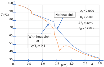
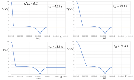
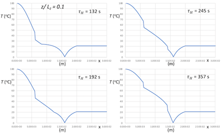
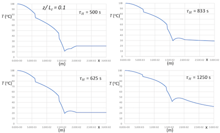
Our second prototype simulations are of heat transfer from a hot body through a layered system, where there is coupling of a highly conductive layer to a cooling bath (shown in Figures 5, 6, 7 and 8), using the parametric model defined by Eqs. 1-6. Note that the cooling layer is not represented explicitly, but phenomenologically. These simulations assume contact conductance between layers, and that heat-sink coupling occurs at one or two of the boundaries along z, as shown in Figures 7 and 8, respectively. As indicated above, the model system, which is 2D, is defined by four boundary conditions. Referring to Figure 5, heat sink boundary conditions at steady state are those of an ambient cooling bath at 42 oC. Referring to Figure 6, heat sink boundary conditions for time-dependent evolution to steady state are those of an ambient cooling bath at 0 oC.

(A)

(B)

(C)

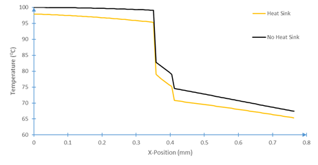
With regards to Figures 5 and 6, the prototype simulations show the results of the multi-layer system in the presence of a heat sink where Figure 5 is a steady state snap shot and Figure 6 is a time evolution of the system. The systems show that the heat sink draws energy and reduces the temperature of the materials in close proximity of the heat sink. This effect propagates through the various mediums, but primarily reduces the temperatures of the mediums farthest from the isothermal boundary condition. The model is qualitatively in agreement with circuit modelling approaches of heat transfer where the energy travels along the path of least resistance, i.e., the energy primarily travels from the hot boundary condition to the heat sink.

Referring to Figures 7 and 8, the model system represented by Eqs. 1-6 is two dimensional and associated with four boundary conditions, which are specified at the heated and outer-surface boundaries, and at the boundaries z = 0 and L_z. Again, the quantity L_z, which for present simulations has arbitrary units, is scaled according to the transverse length l1 coupled to cooling bath (see Figure 1) and the parameter τ_H , is equivalent to the hot-boundary heat flux, is scaled with respect to measurements.

The prototype simulations, whose results are shown in Figures 5 and 6, demonstrate the general procedure for inverse thermal analysis using the parametric model Eqs. 1-6. In reality, a layered material system, heat-sink coupled to a cooling bath, is characterized by contact conductance’s at interfaces between layers (a function of the process used for layering) and anisotropic cooling along and transverse to the embedded heat-sink channel. This anisotropic cooling depends on the nature of heat-sink-layer coupling to adjacent layers and cooling bath. Accordingly, design of a heat-sink-cooled layered material requires quantification of heat-sink coupling that is convenient with respect to inverse thermal analysis. Equations 1-6 defines a parametric model requiring a relatively small number of parameters to be adjusted for encoding thermal response characteristics of embedded heat sinks. In essence, the parametric model Eqs. 1-6 adopts an ideal layered system, having no contact conductance, as an initial ansatz to be further adjusted according to inverse thermal analysis of heat-sink coupling, where delay-time, τ_H, cooling fluxes Q_x, Q_y and Q_z, heat-sink coupling parameter ∆T_c,, are adjustable parameters, and contact diffusivities are determined by inverse thermal analysis. The parametric model Eqs. 1-6 is structured for 3D representation, and thus for the model system considered here, which is 2D, the parameter Q_y = 0.

5. Inverse Thermal Analysis

This section presents an inverse thermal analysis using the parametric model Eq. 1-6. To perform the inverse analysis, a series of temperature measurements must be collected in the system without heat sink coupling to create a series of equations and unknowns for the contact conductance’s and scaling parameters at steady state, Eqs. 14 – 15. It is assumed that contact conductance and the scaling parameters are not a function of time or heat transfer; thus, the model is analyzed at steady state. Due to the full length of Eq. 1-4, each complete equation for the specified boundary condition will be similarly separated into four pieces.

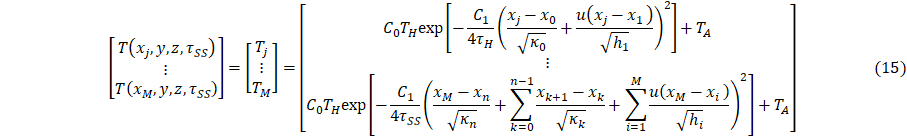
And

With the parameterization of Eq. 1, the heat sink can be coupled to a cooling to bath parameterize the heat sink terms, Q_x, Q_y, and Q_z, where the heat sink temperature change, ∆T_c, is experimentally measured. The quantities Q_x, Q_y, and Q_z are determined through a three point calibration. This results in a system of three equations and three unknowns, Eqs. 15-18. Due to the full length of Eq. 1-4, each complete equation for the specified boundary condition will be similarly separated into four pieces.

6. Prototype Inverse Thermal Analysis

This analysis demonstrates the thermal response properties between layers and heat-sink coupling with an emphasis on analysing a system with varying contact conductance between the layers. Because of their nature and the complexity as a function of specific system designs, the parametrization is not readily available based on formal thermal properties previously determined; therefore, the parameters must be determined inversely. For the purposes of this inverse analysis, a single multi-layer material comprised of Nyco and copper will be considered where the copper acts as an embedded heat sink between two layers of Nyco. The material properties are listed in Table 1 which have been experimentally determined.

Table 1. Material properties for the cotton, copper, and Nyco system.

	t [mm]	𝜌 [Kg⸱m-3]	k [W∙m-1∙K-1]	Cp [J⸱kg-1⸱K-1]	[m2∙s-1]
Copper	0.051	8960	391.2	389.4	1.112⸱10-4
Nyco	0.356	5.07	15.4	1445	2.102⸱10-3

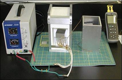
To simplify the mathematical model and experimental test setup, a small sample with a cross section of 3 cm by 3 cm was evaluated where the temperature variation along the y-axis and z-axis were considered negligible. Additionally, the system was evaluated by sandwiching the samples in between an isothermal hot plate and cold plate where the system is tested with and without heat sink coupling, Figure 9. Due to the test setup, the radiation component was considered negligible. The resulting temperature data is listed in Table 2.

The experimental setup, Figure 9, has additional error sources; however, those error sources are inconsequential with respect to the validation of the parametric model. First, the experimental setup uses weighted blocks to compress the material stacks such that the contact between layers is consistent and repeatable – the physical contact between layers directly influences the thermal contact conductance between the layers. The second source of error stems from the thermistors and thermistor measurement controller. It is assessed that the thermistor and thermistor measurement controller combination have <0.1°C of temperature accuracy and variation based on previous validation measurements not discussed in this paper. For the isothermal hot-plate, the temperature is controlled by a PID controller to minimize variation. Additionally, the hot-plate is allowed to reach temperature prior to inserting the material and starting the experimental test. The final notable sources of error are the ambient environmental temperature and water bath temperature which were continuously monitored. Overall, these various sources of error are small with respect to the global temperature measurements within the material. Additionally, the model is parametrized via measurements using this machine such that errors of the machine measurements would equally present themselves in the model, but the relative error between the model and measurement would be consistent.

(A)

(B)

(C)

Table 2. Thermal testing for the cotton, copper, and Nyco system where a is the Hot Plate Temperature [^oC], b is the Interface 1 Temperature [^oC], c is the Interface 2 Temperature [^oC], and d is the Cold Plate Temperature [^oC].

	[s]	a [oC]	b [oC]	c [oC]	d [oC]
No Heat Sink	0	100.0	19.1	18.7	18.7
No Heat Sink	1000	100.0	83.0	78.8	67.4
Heat Sink	0	100.0	19.1	18.4	18.4
Heat Sink	1000	100.0	85.2	74.8	65.3

The thermal measurement results can be used in conjunction with Equations 13-18 to parametrize the system via inverse analysis, which yields the basis function coefficients (C₀ and C₁) and heat flux (Q_x), Table 3. This analysis assumes a 1-D mapping of the 3-D system such that the y and z component variation, Q_y and Q_z, is considered negligible; thus, evaluating to one. This results in Eq. 16’s simplification into Eq. 20.

Table 3. Parameterization of the Nyco-Copper-Nyco system.

System Parameter	Parameterization Values
C0	0.2179
C1	7.2982∙105
h0	1252.9193
h1	48533.7643
Qx[K∙m-1]	0.1934
∆TC[K]	4.400

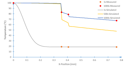
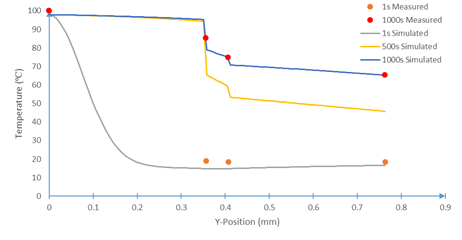
Using the parameterization, the thermal model, Eqs. 1-4, can be evaluated to show the time evolution of the temperature fields with and without heat sink coupling, Figures 10-12. Note that position zero represents the hot boundary, and the position 0.8 mm represents the cold boundary.

7. Discussion

The parametric model defined by Eqs. 1-6 is a formal adaptation of the heat-kernel solution of the heat-conduction equation for simulation of heat-transfer in layered materials, which are coupled to heat sinks at edge boundaries. As described schematically in Figure 1, the model is of a three-dimensional system that approximates heat-sink cooling of a heated layered material. The purpose of which is to handle the multi-scale nature of thin layered composites with embedded heat sinks. The parametric model combines both energy-transport through an ideal system of layered materials, not having contact conductance, representing the model ansatz, and phenomenological parameterization for the influence of contact conductance and embedded heat sinks. The parametric model, whose construction is according to physical theory, includes the phenomenological source function f(x,y,z) representing multiscale coupling of embedded heat sinks, where cooling baths are located at edges of the system. Formulation of the source function f(x,y,z) is based on the approximation defined by Eqs. 11 and 12, which is formally reinterpreted with respect to a cooling flux at a boundary. This function is structured for encoding of thermal response associated with anisotropic heat transfer at steady state. Determination of anisotropic heat diffusion characteristics poses a problem for inverse thermal analysis. In the spirit of inverse analysis, parameterization of the model is not unique, but adapted for convenience.

The parametric model Eqs. 1-6 poses the problem of generating a parameter space that is sufficiently dense, expansive and bounded, for extraction of estimated parameter values for a given target layered system. Given a parameter space, estimation of target parameter values may be achieved by observation of parameter trends as a function of quantities characterizing a class of layered materials, e.g., material combinations, thickness, contact conductance, heat-sink properties. Estimation of target parameter values can also be achieved using algorithms for searching within parameter spaces. Selection of appropriate parameter-search algorithms poses a problem itself, which should depend on the form of the parameter space.

Constructing the prototype experiment inverse analysis above exposed the singular nature of the heatsink and contact conductances relative to the other layers. It is apparent from Figures 10-12 that there the model has excellent agreement with experimentally measured data, but there is a significant contact conductance singularity between the layers despite pressing the system together. This is to be expected as the contact conductance parameter encapsulates not only the insulated effect of poor layer contact, but also the reflected and transmitted heat waves not expressly given by this model.

8. Conclusion

Determination of optimal process parameters for achieving a given target temperature field for heat transfer through a layered material using material-layer configurations and heat sinks poses a specific problem. The results of this study demonstrate use and general features of a parametric model, which can provide estimation of heat-transfer characteristics for layered materials coupled to heat sinks while handling both the singular nature of the contact conductance’s and heat sinks. The nature of this model is that a singular basis function is used to represent the layered system while inverse analysis is performed at steady state. The model can be further modified to include a full basis function representation of all the layers using a discrete number of basis functions greater than one. This inherently will provide better estimation and agreement with experimentally measured results, but the increased complexity will complicate inverse thermal analysis. Additionally, as mentioned in the discussion, the contact conductances of this model inherently include the reflected and transmitted heat waves within the system. Thus, the model can be further modified to explicitly call out those parameters such that it further isolates only the effects of poor material contact between layers. Overall, the model, as presented in this analysis, provides sufficient agreement between experimentally measured data and simulated data for the analysis of thin, multi-scale materials. The next steps will be to include more complex effects within the model and expand the number of basis functions to represent the time evolution of the fields.

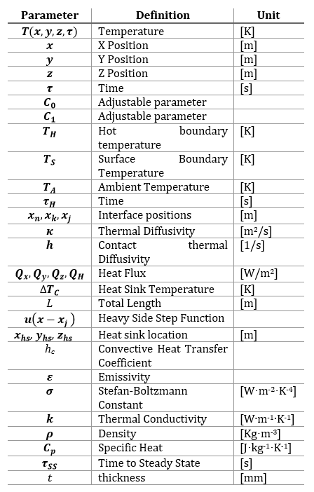
9. Nomenclature

For brevity of the document, this nomenclature section outlines the various variables present in the parametric model and associated equations.

References

[1] S.G. Lambrakos, Parametric Modeling of Welding Processes Using Numerical-Analytical Basis Functions and Equivalent Source Distributions, Journal of Materials Engineering and Performance, Volume 25(4), April 2016, pp. 1360-1375. View Article
[2] E. Michaelchuck, S. Ramsey, T. Mayo, S.G. Lambrakos, Experimental Proof of Concept for Heat Sink-Controlled Temperature Fields within Multi-Layered Materials, U.S. Naval Research Laboratory Memorandum Report, U.S. Naval Research Laboratory, Washington, DC, NRL/MR/5708--20-10,100, October 11, 2020.
[3] H. S. Carslaw and J. C. Jaegar, Conduction of Heat in Solids, Clarendon Press, Oxford, 2nd ed, 374, 1959.
[4] A. Tarantola, Inverse Problem Theory and Methods for Model Parameter Estimation, SIAM, Philadelphia, PA, 2005. View Article
[5] M.N. Ozisik and H.R.B. Orlande, Inverse Heat Transfer, Fundamentals and Applications, Taylor and Francis, New York, 2000.
[6] K. Kurpisz and A.J. Nowak, Inverse Thermal Problems, Computational Mechanics Publications, Boston, USA, 1995.
[7] O.M. Alifanov, Inverse Heat Transfer Problems, Springer, Berlin, 1994. View Article
[8] J.V. Beck, B. Blackwell, C.R. St. Clair, Inverse Heat Conduction: Ill-Posed Problems, Wiley Interscience, New York, 1985.
[9] J.V. Beck, Inverse Problems in Heat Transfer with Application to Solidification and Welding, Modeling of Casting, Welding and Advanced Solidification Processes V, M. Rappaz, M.R. Ozgu and K.W. Mahin eds., The Minerals, Metals and Materials Society, 1991, pp. 427-437.
[10] J.V. Beck, Inverse Problems in Heat Transfer, Mathematics of Heat Transfer, G.E. Tupholme and A.S. Wood eds., Clarendon Press, (1998), pp. 13-24.B. Klaus and P. Horn, Robot Vision. Cambridge, MA: MIT Press, 1986. View Article