Journal of Fluid Flow, Heat and Mass Transfer (JFFHMT)

ISSN: 2368-6111

Characterization of the Turbulent Fluid Flow Structures in a Slab Mold with Experimental Measurements and Different Turbulence Models

M.G. González-Solórzano¹, S. García-Hernández ², R.D. Morales ¹, A. Nájera-Bastida³, Javier Guarneros⁴

¹Intituto Politécnico Nacional-ESIQIE, Department of Metallurgy,
Ed. 7, Zacatenco, Mexico City, 07738
mgonzalezs2007@alumno.ipn.mx; rmorales@ipn.mx
²TecNM-Instituto Tecnológico de Morelia, Metallurgy Graduate Center,
Av. Tecnológico No. 1500, Morelia, Michoacán, México, 58120
saul.gh@morelia.tecnm.mx
³Instituto Politécnico Nacional-UPIIZ, Metallurgy Engineering,
Blvd. Del Bote 202, Cerro del Gato, Zacatecas, México, 98160
alfonso_najera@yahoo.com.mx
⁴K&E Technologies, Department of Investigation,
Manizalez 88, San Pedro Zacatenco, México City, 07365
javier.guarneros.g@gmail.com

Abstract - The turbulent flow of liquid steel in a slab mold was characterized using a commercial nozzle through physical water-model experiments and four turbulent models: k-ε Realizable (RKE), Detached Eddy Simulation (DES), Scale-Adaptive Simulation (SAS), and Large Eddy Simulation (LES). The comparison between numerical results and the experimental measurements (using Ultrasound Velocimetry) permitted the characterization of flow structures along a sub meniscus region, (of great importance for flux-dragging phenomena) In general, all four models predict characteristic unsteady state turbulent flows. However, the k-ε Realizable and DES models fail to predict instabilities in the internal flow of the nozzle, overpredicting sub-meniscus velocities in the mold. On the other hand, the SAS and LES models manage to predict the instabilities and changes in the internal flows inside the nozzles that occur at high frequencies and achieve an excellent agreement with the experimental velocity profiles. With the analysis of the results obtained, it is possible to say that the SAS model produces performances like those of the LES model with less computing effort and less cost.

Keywords: Turbulent flow, Turbulence models, Turbulent characterization, Fluid flow structure, Meniscus region.

© Copyright 2024 Authors - This is an Open Access article published under the Creative Commons Attribution License terms Creative Commons Attribution License terms. Unrestricted use, distribution, and reproduction in any medium are permitted, provided the original work is properly cited.

Date Received: 2023-11-01
Date Revised: 2024-01-26
Date Accepted: 2024-02-08
Date Published: 2024-02-29

1. Introduction

Fluid flow structures in steel slab continuous casting molds are most important as they define product quality and caster productivity. Turbulent conditions driven by the discharging liquid jets originate from unsteady flows characterized by vortexes and eddies with a broad spectrum of sizes and energies. Uncontrolled flows lead to slab defects like slivers formed by the dragging action of mold powder due to high, near-meniscus liquid velocity [1]-[3]. Heat transfer and shell solidification patterns may induce longitudinal cracks [4], [5], and strand breakouts originate in the region of the gap between the nozzle and the mold wall due to uneven heat fluxes [6]-[8]. Addressing the dynamics of turbulent flows in the mold is the motive of reports and publications using physical models and mathematical simulations. Vanka et al. [9], [10] characterized these flows through simulations using the Direct Navier-Stokes (DNS) approach [11], [12] and Particle Image Velocimetry (PIV) measurements of velocity fields in a water model. Their report provides the finest structures yielded by the DNS of the flow exceeding the resolution of the PIV fields. However, the computer requirements are only available for scientists in the turbulent flow area. S.M. Cho et al. [11] built a combined mathematical model consisting of the Large Eddy Simulation (LES) [13] and the Volume of Fluid (VOF) [14] to study the transient flow and the slag behavior during the casting time. The authors reported severe irregularity and unsteady flows using upwards port angles. Yuan et al. [15] used a 0.4 downscaled water model to test the reliability of the LES model to predict the velocity fields determined through PIV measurements finding a good matching.

The studies related to direct performance comparisons between different turbulence models applied to fluid flow in the molds are scarce, though there are important contributions oriented to this task. Choudhary et al. [16] tested the LES model against two RANS models, the standard k-ε model (SKE) [17] and the Realizable k-ε model (RKE) [18]. The three models were tested against measurements of velocity fields using PIV techniques in a downscaled water model (0.4 scale). They found that the LES model outperforms the SKE and RKE models in their prediction capabilities of the velocity fields, and the SKE model does it over the RKE model. These last findings contradict the work of Gonzalez-Solórzano [19] who reported that the RKE model predicts well the experimental unsteady state velocity fields in a full-scale water model. (Lan et al. [20] applied six k-ε models [17], [21]-[24] to the experimental fluid flow data of a billet mold water-model obtained through Laser Doppler Velocimetry techniques (LDV). Their findings report that the low and high Reynolds numbers predict the trends of the axial velocities and the associated kinetic energy. However, the low Reynolds number model outperformed the high Reynolds number model in the predictions of turbulent kinetic energy. In regions out of the axial positions. In general, the model Chien [24] provided consistent results, and the errors, compared with the experimental measurements, were among the smallest. Kratzsch [25] tested the performances of the Unsteady Reynolds Averaged Navier-Stokes models (URANS) models such as the SKE [17], the RNG k-ε [26], the RKE [18] and the SST k-ω [27]. The authors claim a reasonable agreement with the experimental averaged velocity and the structure of the flow with any of these models. However, the RNG k-ε and the k-ω SST model using second-order discretization schemes rendered the most accurate results. Gregorc et al. [28] used a billet full-scale water model and PIV technique to test the flow structure prediction capability of the model RKE [18], SST k-ω [27], the scale resolved LES [13] and hybrid Scale Adaptative Simulation (SAS) models [29]. Their results indicated that the four models yielded acceptable predictions of velocity fields. There is no appreciable flow structure dependence on time, even when using unsteady RKE and SST k-ε models. The SAS and LES models render unsteady flows through all the simulation time.

The present work deals with the fluid flow structure of liquid steel in a continuous casting slab mold, testing the RKE, LES, DES, and SAS models against the experimental flow structure characterization performed along a sub meniscus region using Ultrasound Velocimetry techniques. Various goals are on sight:

1. The capability of the RKE to predict unsteady fluid flow conditions.
2. The quantification of the gap between a RANS model and a scale-resolved LES model.
3. Assessment about the possibility of using the SAS model over more demanding computing efforts like the LES model.
4. The performance of the DES model compared with resolved scale and RANS models.

The following lines provide detailed explanations about the frame of the work, the experimental and mathematical approaches, the discussion, and the conclusions.

2. Turbulence Models

2.1. The k-ε Realizable Model

The Realizable k-ε Model (a Reynolds Averaged Navier-Stokes, RANS Model) can predict complex flows [18]. The key feature of this turbulence model is the combination of the Boussinesq relationship with the classical eddy-viscosity definition [30] expressed by the following expression for the normal Reynolds stresses corresponding to an incompressible strained flow,

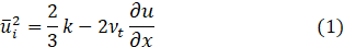
the turbulent viscosity ν_t=μ_t⁄ρ permits the calculation of the normal stress given in Equation (1). This stress should be a positive quantity. However, it can be negative, i.e., "non-realizable," when matching the following condition for the strain rate:

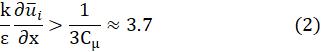
Thus, under these conditions, the Schwarz inequality [31] expressed by (Einstein's rule does not apply to α and β) (3)

is violated when the mean strain rate is large. The advisable way to avoid negative normal stresses and the violation of the Schwarz inequality is to make the “constant” C_μ a variable sensible to the mean deformation rate quantified by the k and ε fields, as explained below.

Therefore, the equations of continuity and momentum transfer and the equations of turbulent kinetic energy and its dissipation rate are the following.

Considering water as an incompressible fluid, the mass continuity equation is,

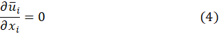
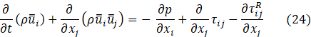
The corresponding balance of momentum is,

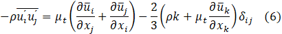
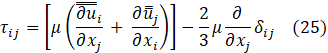
The equations (4)-(5) form an unclosed system since the penultimate term, known as the Reynolds stresses, would require another six equations for completeness. To close the system, the turbulent viscosity hypothesis through the Boussinesq expression [32] lets writing these stresses as,

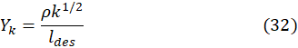
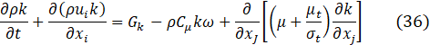
the turbulent kinetic energy, k, and its dissipation rate, ε, balances are.

Where Y_k=ρε, the dissipation rate of the kinetic energy.

The pseudo constant C₁ is maximized among the following set,

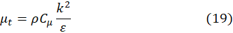
The turbulent viscosity is calculated, as in all k-ε family models, by

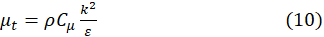
However, the difference between the realizable k-ε and the standard k-ε (SKE) and RNG k-ε models is that the C_μ is no longer a constant. Instead, it is computed from the following expression.

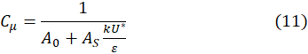
where,

and

is the mean rate-of-rotation tensor seen from a moving reference frame with the angular velocity ω_k, and  is the Civi-Levita symbol. The model constants A₀ and A_S are as follows:

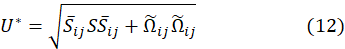
The parameters of the model have the following expressions:

(16)

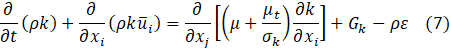
The term G_k, in Equation (7), is the production of the turbulent kinetic energy originated by the interaction between the Reynolds stresses and the mean flow (following the Boussinesq hypothesis) given by,

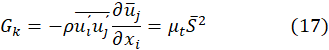
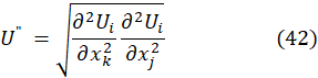
where .The mean deformation rate tensor is

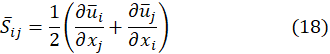
Once knowing the fields of k and ε is possible to calculate the turbulent viscosity through

The model constants have the following values: C_1ε=1.44, C_2ε=1.92, σ_k=1.0, and σ_ε=1.2.

The RANS models, such as the RKE model, have two main characteristics, the computed fields are averaged in time, missing the effects of the turbulent fluctuations- Second, the capture of the turbulent flow structure, including the smallest eddies, is not possible even using very small mesh sizes at a high computing cost. Hence, other models for studying the flow structures are in demand if required.

2.2. The Large Eddy Simulation (LES) Model

Turbulent flows have wide ranges of length and time scales, and the largest eddies have sizes comparable to the characteristic length of the mean flow. In contrast, the smallest eddies dissipate the turbulent kinetic energy. The large eddies transport momentum, mass, energy, and other passive scalars. Their sizes depend on the system's geometry and the specific boundary conditions. The smallest eddies are less dependent on the geometry and size of the system, are isotropic, and hence more universal. The latter feature allows for finding a universal turbulence model for these smallest sizes. Therefore, the approach used by the LES model consists of proceeding with the simulation of the large eddies and modeling the smallest eddies. The discrimination between large and small eddies is possible through the mathematical filtration of the continuity and momentum equations. The filtration of a variable ϕ is.

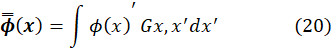
in terms of the finite volume computational scheme, the filtration of this variable is.

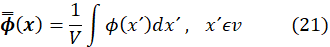
Where V is the volume of the computational cell, implicitly the filtration function G(x,x)' is

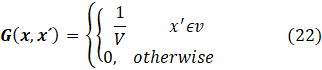
thus, filtering the Navier Stokes equations using (21) yields,

The stress tensor due to the viscous momentum transfer is,

The sub-grid-scale stress tensor is

These stresses, like the Reynolds stresses, are unknown. Therefore, the Boussinesq hypothesis is helpful again to close the system in its version:

The filtered strain rate tensor will be.

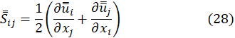
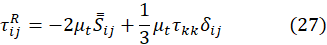
To calculate the turbulent viscosity employed in the computations of the residual stresses in Equation (27), the Wall-Adapting Local Eddy-Viscosity (WALE) model is preferable over the Smagorinsky and Smagorinsky-Lilly models [33]

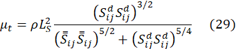
where L_S and S_ij^d in the WALE model are,

where V is the computational cell volume.

2.3. The Detached Eddy Simulation (DES) Model

This hybrid model combines a RANS model in the boundary layer flow and the LES for the outside of this flow. The LES region is associated with the core of the turbulent, where large and unsteady eddies dominate the transport of kinetic energy. In the boundary layer where viscous stresses dominate, eddies become smaller, dissipating the kinetic energy, and the RANS model is more appropriate to diminish the number of computing cells. Therefore, the DES model deals with high Reynolds wall-bounded flows without the high cost of the LES model resolving the near-wall with fine computing meshes demanding large memory capabilities.

In the present work, the RANS model of choice is a modified Realizable k-ε model, described above, to simulate the near-wall flow. The modification consists of using a different dissipation energy term Yk in the balance of k:

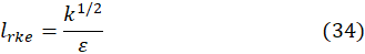
Where C_des is a constant with a value of 0.61, and Δ_max is the maximum local mesh spacing (Δx, Δy, Δz). When l_des=l_rke, the term of dissipation rate Y_k of Equation (7) is recovered.

2.4. The Scale-Adaptive Simulation (SAS) Model

The SAS model damps the resolved structure at high wavenumbers (the smallest eddies) of the kinetic energy spectrum until the limit resolution of the mesh. The main unknown of the turbulent kinetic energy balance is the dissipation rate of kinetic energy, ε, and its determination requires the solution of another transport equation. Therefore, the turbulent kinetic energy, k, is fundamental to determining the flow structures whose transport equation includes the dissipation rate of the kinetic energy, , in conventional URANS models. For example, in the k-ω turbulence model, ω ( , the eddy frequency) is modeled under analogy to the k equation (is the same for the balance of ε in the k-ε models) using purely dimensional and heuristic approaches. Instead of using the same approach [34], Rotta [29] derived a balance for the product between the kinetic energy and the integral length scale, kL. However, Rotta introduced a third-order derivative of the velocity field in his derivation, leading to difficulties and tedious procedures in implementing this derivative into CFD codes. To avert this condition, Egorov and Menter [29] modified their SST model to become the SST-SAS model, deriving balances for k and ω according to:

The generation of the turbulent kinetic energy is, G_k=μ_t S². The main difference between the SST-RANS and the SST-SAS models (or simply, the SAS model) is the term Q_SAS; σ_ω2 and σ_ω are the same as the SST model. The Q_SAS term is:

This SAS source term originates from a second-order derivative in Rotta's transport equations, including a source/sink term.

The computing of the integral scale in the SAS model is through the previous knowledge of the k and ω fields,

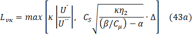
The Von Karman length scale, L_vκ (a three-dimensional generalization of the classic boundary layer theory of Schlichting) [35], helps to evaluate the local flow degree of inhomogeneity. Its 3D expression is like that given for the hydrodynamics of a boundary layer:

where,

The model constants are η₂=3.51,σ_Φ=2/3,and C=2. In the logarithmic-law part of the boundary layer, the von Karman constant is κ=0.41 and thus L=L_vκ. The model controls the high wavenumber damping through the following expression:

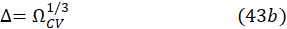
Ω_CV is the control finite volume size. This limiter is useful to damp the finest resolved turbulent fluctuations. The equilibrium eddy viscosity, derived from a balance between the production and destruction of the kinetic energy, is:

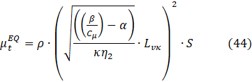
The structure of this formula is very similar to Smagorinski's sub-grid-scale eddy-viscosity of the Large Eddy Simulation, LES model [36]

Therefore, the limiter imposed on the magnitude of L_vκ magnitude must prevent the SAS eddy viscosity from decreasing below the LES sub-grid scale-eddy viscosity:

The limiter imposed on the L_vκ value must prevent the SAS eddy viscosity from decreasing below the LES sub-grid-scale eddy viscosity.

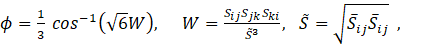
The SAS model identifies the asymmetry of the inhomogeneous flow characterized by large velocity gradients through the Von Karman scale L_vκ; when this scale decreases in the resolved eddies, the ratio (L/L_vκ) increases, making the term Q_SAS a great contributor to the increase in the magnitude of the ω and the ε fields since . These changes are accompanied by the simultaneous decreases of the turbulent kinetic energy, k, and the turbulent viscosity μ_t magnitudes so that the modeled dissipation (i.e., the damping effects) of the turbulent viscosity on the resolved fluctuations is minimal. The regions with fine meshing receive a larger contribution from the Q_SAS term resulting in the generation of turbulence-spectra variables. Besides, the SAS model is a valuable tool for studying the coherent structures of turbulent flows [37]. The velocity fields and the velocity gradient tensor can compute the Q criterion, which helps define the preponderance of rotational or deformation conditions of inhomogeneous flows. Thanks to the structure of the SAS model it became an improved URANS model with a performance, apparently just below or even at the same level as the LES model but with less demanding computing resources and more information regarding the flow structure.

2.5. Boundary conditions and computing parameters

The link between the wall and the outer flow from the boundary layer is through the log-wall function. The no-slipping boundary condition applies to all walls in the system. For considering the presence of the upper layer phase, the shear boundary condition applies on the bath surface. A pressure boundary condition in the outlet governs fluid exit outside the mold. Table 1 shows the computing parameters employed in all four models.

Table 1. Computing procedures and numerical parameters.

	Realizable	DES Model	SAS Model	LES Model
Parameter	Description /Value	Description /Value	Description /Value	Description /Value
Constitutive equation	URANS based on the realizable k-ε model.	Hybrid RANS-LES based on the realizable k-ε model.	URANS and the SST-SAS model.	The LES equations are derived formally by applying a low pass-filter to the Navier-Stokes equations.
Gradient derivates	Green-Gauss node based	Least Squares cell based	Least squares cell based	Green-Gauss node based
Pressure fields	Body Force Weighted	Body Force Weighted	Body Force Weighted	Body Force Weighted
Pressure-velocity couple	PISO	PISO	PISO	PISO
Convergence criterion	0.0001	0.01	0.0001	0.01
Transient formulation	First Order Implicit	Bounded second order implicit	Bounded second order implicit	Bounded second order implicit
Spatial discretization (Momentum)	Second Order Upwind	Second Order Upwind	Bounded central differencing	Bounded central differencing
Mesh type	Unstructured tetrahedral	Unstructured tetrahedral	Unstructured tetrahedral	Unstructured tetrahedral
Nodes	398488	398488	398488	398488
Elements	2276970	2276970	2276970	2276970
Skewness	Average: 0.10852	Average: 0.10852	Average: 0.10852	Average: 0.10852
	Standard Deviation:	Standard Deviation:	Standard Deviation:	Standard Deviation:
Orthogonal quality	Average: 0.92652	Average: 0.92652	Average: 0.92652	Average: 0.92652
	Standard Deviation:	Standard Deviation:	Standard Deviation:	Standard Deviation:

3. Physical Model

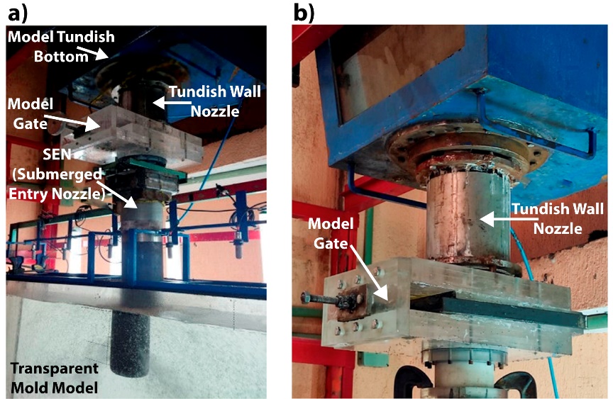
The physical model consists of a full-scale water model of the slab mold made of transparent plastic sheets with dimensions shown in Table 2. The model replicates the existing industrial facility with a tundish holding a steel column of 1 m. The water flows by gravity downwards through the upper tundish nozzle (UTN), which connects with the sliding gate controlling the flow rate through the nozzle and the mold. The fluid is held in a tank below the working floor, equipped with a submerged pump to recirculate the water to the tundish top. A flow meter and a gate valve control the flow rate fed to the tundish in the vertical pipe transporting the fluid from the water tank to the tundish. During an experiment, a gate valve and a tundish sliding gate feeding the casting nozzle control the water flow rate provided in the mold. Before making any measurement, the model runs for 15 minutes until reaching a steady condition; then, the velocity measurements start. Figure 1a is a general view of the complete full-scale model, and Figure 1b is a close view, including the UTN and the sliding gate.

Table 2. Mold Dimensions.

Description	Value (m)
Height	1.7
Width	1.45
Thickness	0.25

The meniscus region of the liquid in the mold requires minimum level variations to maintain the slab surface free of surface cracks [38]-[40]. Thus, the flow structure in this region is significant. Therefore, a drilled hole, located at 20 mm below the static level of the liquid and practiced in the midface of one of the narrow mold faces, holds a 10 million Hz transducer to measure the instantaneous velocities along an imaginary line going from the mold narrow face to the outer nozzle wall. Figure 2 shows the experimental configuration. A set of selected points 1, 2, 3, 4, and 5 assist in characterizing the flow statistics. The software acquires the velocity files and transforms them into flow statistics like average, standard deviation, skewness, kurtosis, power spectra, and auto/cross-correlations. Figure 3 shows the geometric dimensions of the nozzle tested in this work. Table 3 also shows the mold's operating conditions.

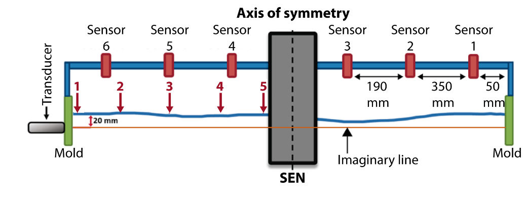
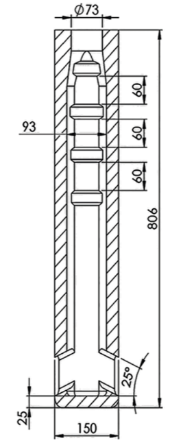
Table 3. Physical properties and experimental conditions.

Parameter	Value
Casting speed, (m/min)	1.4
Liquid flow rate, (l/min)	8.56
Nozzle immersion, (m)	0.120
Valve opening, length, (m2)	2.57x10-3
Pressure inlet, (Pa)	101 325
Water viscosity, (Pa s)	0.001003
Water density, (kg/m3)	998.2

4. Results and Discussion

4. 1. General Fluid Flow Fields

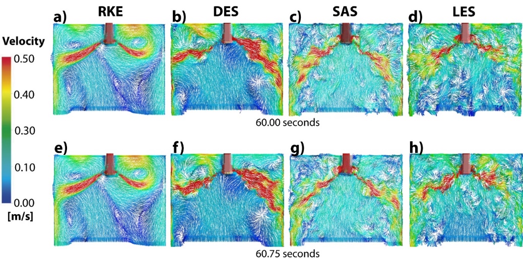
Figures 4a-4d shows the unsteady velocity profiles at the symmetrical-vertical plane of the mold predicted by the RKE, DES, SAS, and LES models, respectively. Figures 4e-4h show the velocity profiles ¾ a second later using the same models. The RKE model yields compact discharging jets with RANS-type velocity fields, without changes visible after such a short period, specifically at the top of the upper roll flows. The right-side, upper roll flow yields the highest magnitudes in the velocity scale. Although, as reported in another work, this model can predict well appreciable velocity changes in the mold after longer periods [41]. The DES model predicts more dispersed discharging jets than the RKE model, matching more closely the experimental observations of the jets revealed through the injection of a red dye tracer, as seen in Figures 5a-5d. There is a high velocity with a magnitude close to the maximum on the velocity scale in the upper roll flow on the left side. By comparing Figures 4b and 4f, it is evident that this model can detect the flow pattern changes after short times, such as ¾ of a second. See, for example, the left and right mold sides. The right side shows a thicker and shortened discharging jet after the mentioned period. The lower roll flows predicted by this model yield streamlined characteristics. On the other hand, the SAS model has a large sensitivity to detect changes in the fluid flow field after a period of ¾ of a second, as observed in Figures 4c and 4g. Far from the characteristics of a RANS model, this model reproduces the instantaneous velocity fields in the upper and roll flows. The velocity fields near o close to the bath surface reported by this model are not as high as those predicted by the former models. The predicted lower flow rolls yield streamlined patterns. It is hard to say that the flow fields predicted by the LES model, Figures 4d and 4h exceed the performance predicted by the SAS model, Figures 4c and 4g. The LES model generally predicts slightly higher upper roll velocities in the near bath surface at both sides of the Submerged Entry Nozzle (SEN) than the SAS model. The lower roll flow model is very unstable, and after the short-mentioned period, it becomes streamlined. Again, the LES model resembles, like the DES and SAS models, the fluid flow patterns of frayed discharging jets observed in Figures 5a-5d.

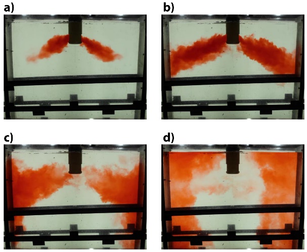
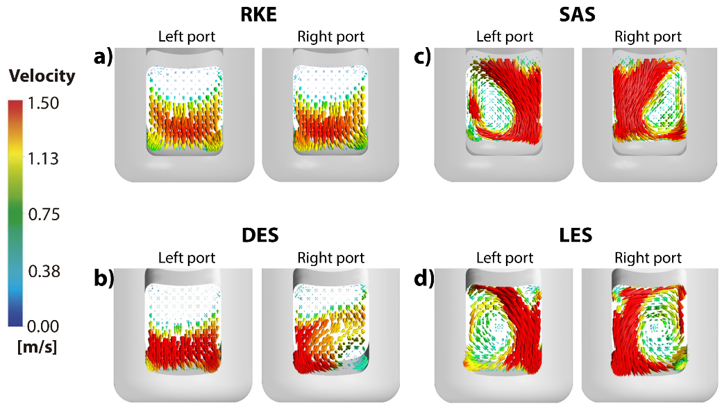
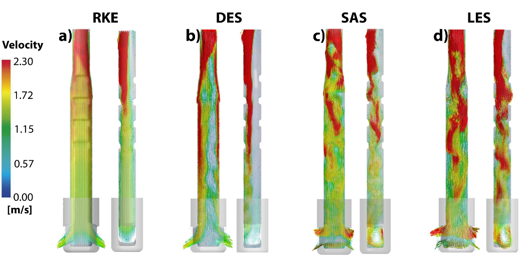
Figures 6a-6d show the outflow patterns of the liquid through the right and left nozzle ports using the RKE, DES, SAS, and LES models, respectively. The RKE and DES models predict unused flow areas in the upper side of both ports, while the SAS and LES model predict swirling clockwise and counter-clockwise flows leaving the nozzle. These effects originate in the opening pattern of the sliding gate reported in Figures 7a-7d for the RKE, DES, SAS, and LES models. The RKE model yields an unchanged flow pattern after a very short period of 0.25 seconds, (it is important to mention that said statement is made since velocity vectors were analyzed every 0.25s of each model, managing to see the changes in the velocity field in such short time periods, reaching the previous statement). The RANS velocity field inside the nozzle reports the highest downward velocity on the side where the opening side of the sliding gate is. The streamlined pattern on the other side, opposite to the highest stream velocity, is not anymore observed in the flow field predicted by the DES model being substituted by a time-changing flow. Unlike the precedent RKE and DES models, the SAS and LES models have the sensitivity to predict changes in the internal fluid flow patterns of the nozzle during very short times. Therefore, intuitively, a turbulent flow inside the nozzle must yield short-time-changing flow fields such as those predicted by the SAS and LES models.

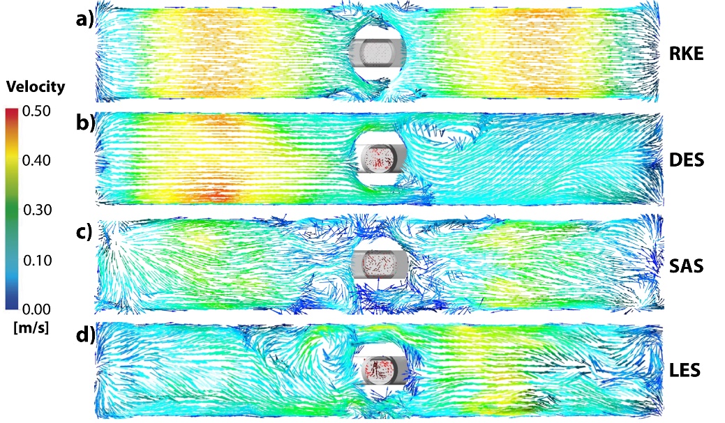
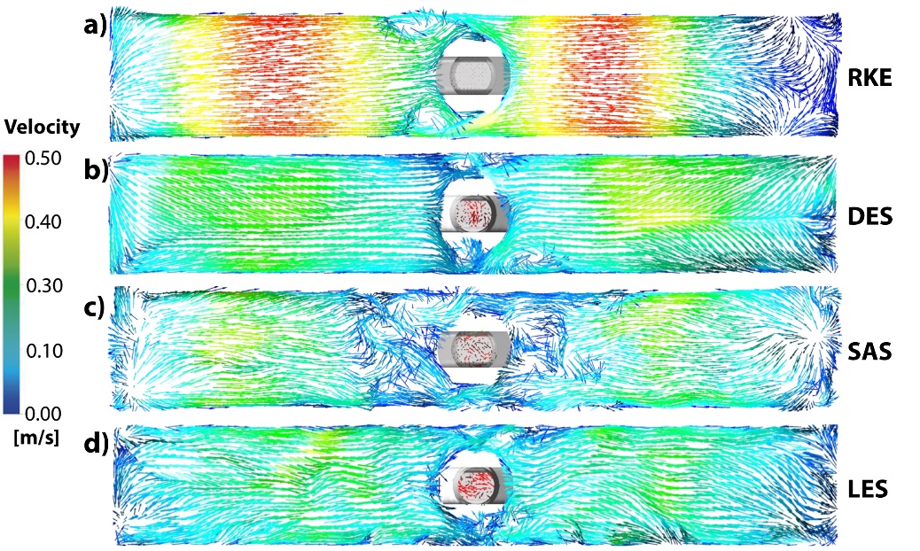
Figures 8a-8d shows the velocity vector field calculated through the RKE, DES, SAS, and LES models at the horizontal plane in the mold 20 mm below the bath surface at 20 seconds of simulation. Figures 9a-9d show the same information 80 seconds after the fields shown in Figure 8, it is worth mentioning that the times mentioned above are after reaching the steady state. Comparing both figures allows us to make the following comments,

• The RKE model tends to yield quasi-symmetric flows. The flows close to the narrow mold faces show minor disorder, and the liquid's velocity vectors emerge smoothly to form the upper roll flow
• The DES model predicts non-symmetric flows, which aligns with the observations of the tracer injected in the water model.
• Unlike the precedent two cases, the SAS model yields vortex flows surrounding the nozzle while the flows in the proximities of the mold's narrow faces look chaotic. The remoteness from the symmetric flow is also a result of this simulation.
• Similar comments from the results of the SAS model apply to the fields predicted by the LES model. The vortex flows surround the nozzle.

4. 2. Comparison between the Experimental and Numerical Results

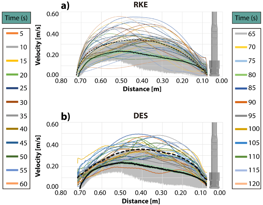
The line traced between the mold's narrow wall and the nozzle, described in the experimental section, works to compare the experimental and numerical results, see Figure 10 and 11. A shadowed gray region indicates the amplitude of the velocity profiles or standard deviations corresponding to the measurements, and black curves are the average of the measured velocities. The interrupted black curves correspond to the numerical averaged velocity profile. Figures 10a and 10b for the RKE and DES models, respectively, and Figures 11a and 11b for the SAS and LES models follow the same description. Each of the curves, plotted on the gray region, are the instantaneous velocities profiles with differences of five seconds, as indicated by the color’s scales in each curve. The RKE model overpredicts the velocities in the near meniscus region, as seen in Figure 10a. Many numerical velocity profiles fall outside the gray experimental area, yielding a numerical averaged profile that matches the gray region's upper boundary. Although, the maximum difference between the numerical and experimental averaged velocities is about 0.10 m/s. The DES model, Figure 10b, yields similar results, and the same comments are applicable in this case. The velocity profiles predicted by this model do not follow the smooth shapes observed in the results presented in Figure 10a. Indeed, Figures 8a-8b and 9a-9b show that velocities predicted by the models RKE and DES models are higher than the velocities predicted by the SAS and LES models in Figures 8c-8d and 9c-9d.

The numerical predictions using the SAS model fall mostly inside the gray area corresponding to the standard deviations of the experimental velocities, providing higher reliability than the two precedent models. The averaged numerical and experimental velocity profiles do not have a perfect match. However, it is fair to say in favor of the SAS model, the same as the LES model, that the experimental and computational times do not coincide, which makes a difference. The LES model also predicts velocity profiles falling mostly inside the gray experimental area, and the numerical and experimental averaged velocity profiles mismatch slightly in the region close to the nozzle. Both models, SAS, and LES, predict non-smoothed velocity curves obeying the instantaneous nature of the turbulence.

4. 3. Turbulence Characterization

Characterizing the turbulent flow in the proximities of the meniscus in slab mold is helpful to understand the mechanisms involved in the flux dragging phenomena [42]-[44]. The characterization tools used in the present work are autocorrelation, cross-correlation, and Power Spectra Density (PSD). The autocorrelation function, a normalized autocovariance of the velocity profile along the imaginary line, helps to study the flow structure. This one-point correlation function is expressed by,

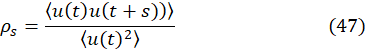
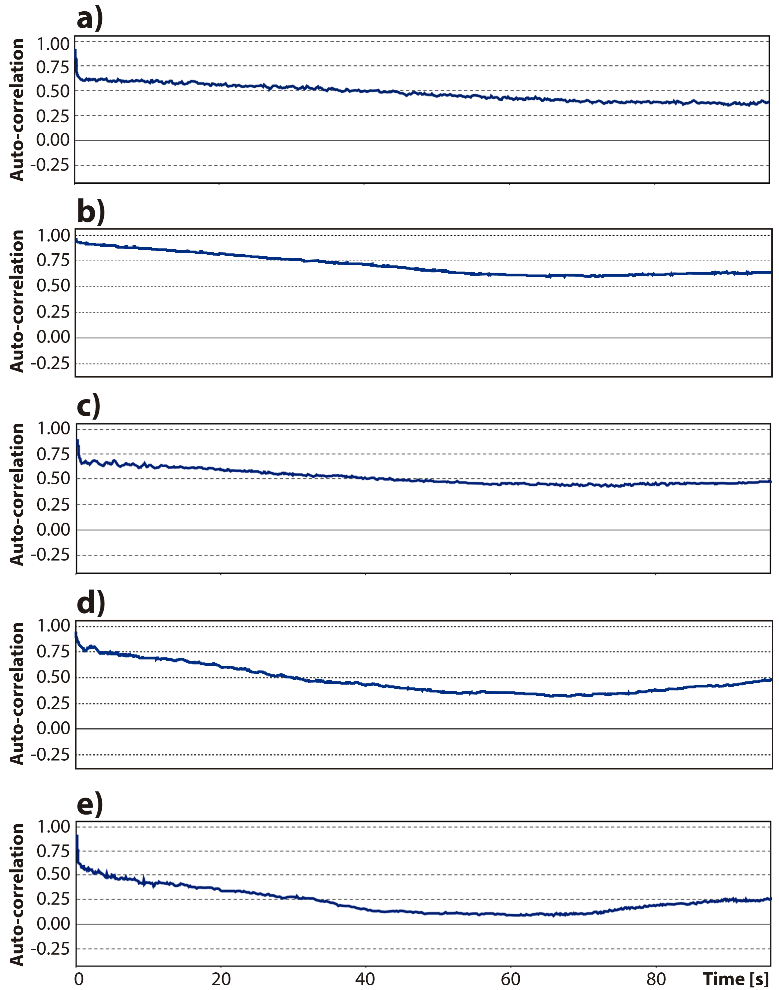
Therefore, applying Equation (47) to the measured velocity files makes possible the calculation of the autocorrelation function for the five points marked in Figure 2. Figures 12a-12e shows the autocorrelations corresponding to these five points. The autocorrelations indicate low-frequency turnarounds of the flow, and they do not decay to the level of zero. Points 4 and 5, the closest ones to the nozzle, yield the largest decay and a later recovery at long times, while the other points remain with relatively high correlations.

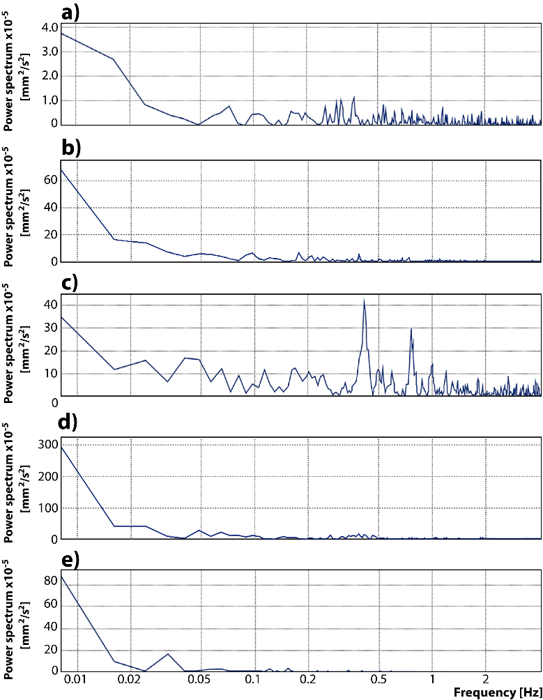
The power spectra density is defined as follows,

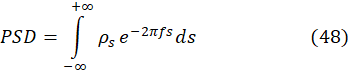
the PSD is the Fourier transform of the autocorrelation function. Regarding the time shifts and the frequency of the random velocities, Figures 13a-13e shows the Power Spectra Density (PSD) corresponding to the five points in the sub meniscus region. The lowest energy is located close to the mold's narrow face, where the velocities have the smallest magnitudes, as seen in Figure 8 and 9. The prominent peaks have very low frequencies, and others have significant frequencies but with very low energies, like points 1 and 3. The highest PSD is in point 4, where the vortex flows near the nozzle (see Figure 8 and 9). Given that point 4 has the highest PSD, discussing the cross-correlations between this point and the other four points is advisable.

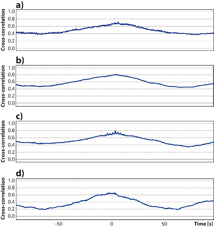
The cross-correlations find relations between two different time series,

the cross-correlation is

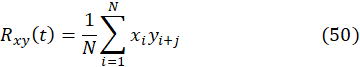
Figure 14 shows this information; as seen there, the highest cross-correlation of about 0.8 at time zero is between points 2-4 and 3-4. All the cross-correlations show a periodical behavior and remain above 0.4, except for the cross-correlation between points 4-5. The effects of the standing wave focused on point 4, with the highest PSD influencing all the autocorrelations in the line.

Finally, the vortex structure complements the characterization structure of the flow through the Q criterion. The Q method involves calculating the complex eigenvalues of the gradient velocity tensor [45]. The Q criterion [46], [47] is appropriate for this work's vortex identification process. The velocity gradient tensor is

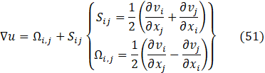
The Q criterion is, therefore,

where , S and Ω are the symmetric and antisymmetric components of the velocity gradient tensor, ∇u. Thus, Q represents the local balance between shear strain rate and vorticity magnitudes.

Figures 15a-15c shows the Q contours calculated by the DES, SAS, and LES models. The positive values mean that the vorticity deformation exceeds the linear dilation deformation. The DES model yields Q fields with magnitudes close to zero, indicated by the green areas. The SAS model predicts strong rotational deformations exceeding the dilation deformations, particularly in the regions approaching the nozzle. Meanwhile, the model LES yields Q intermediate magnitudes between those predicted by the DES and SAS models. The magnitudes of Q near the nozzle regions match the existence of the PSD peaks reported in Figures 13d and 13e.

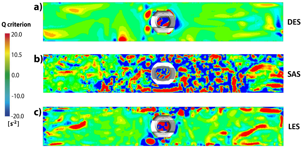
Overall, the performances among the four turbulence models favor the SAS and LES models, followed by the DES and the RKE model in the last place. Table 4 shows the normalized computing times using the same machine. The last two models do not predict the instantaneous velocity fields inside the nozzle. Hence, these odels are helpful as approximations though they remain useful as nozzles design tools when the detail of the flow is not the primary goal. The most important results of these simulations are the performance of the SAS model, which employs fewer computing efforts and provides details of the flow structure and the LES model.

Table 4. Computing time index.

Turbulence Model	Computing time Index	Machine Characteristics
RKE	0.37	Processor: Intel Xeon E5-2650 v4 Cores: 12 Logical Processors: 24 Frequency: 2.20 GHz Ram: 16Gb, 2400MHz System Type: 64-bit Operating System · Windows 10 Pro Operating System, 20H2 Graphics card: NVIDIA Quadro K420, memory (VRAM) 2007 MB. Storage Type: HDD
DES	0.58
SAS	0.73
LES	1.00
Note: The longest time for the LES model has the index base of 1.

Based on the results obtained, it could be said that there are certain limitations, especially with the RKE and DES models, since these two models, despite predicting the unstable flow conditions in the mold, fail to predict the same conditions within the nozzle, they omit the flow structure. Furthermore, they overpredict velocity measurements in the meniscus area, which limits decision making, leading to wrong decisions due to the magnitudes obtained and the omission of the flow structure.

5. Conclusions

The performances of four turbulence, RKE, DES, SAS, and LES models are tested against the turbulence measurements in a full-scale water model of slab continuous casting mold. The conclusions derived from the results and the discussion of these activities are as follows:

• The four models predict the unsteady state conditions characteristic of turbulent flows. Though, the RKE model requires longer times, such as one second, to detect changes in the flow patterns in the mold.
• The RKE and DES models cannot predict the unsteady conditions inside the nozzle mold. The SAS and LES models predict fluid flow pattern changes with frequencies as high as 4 s-1.
• The RKE and DES models overpredict the velocity field measured along a subsurface line 20 mm below the bath surface, starting from the midface of the narrow wall mold to the nozzle. The SAS and LES models match very well the experimental velocity profiles. The SAS model performs similarly to the LES model with smaller computing efforts.
• The autocorrelation-velocity profiles along the measuring line do not reach zero even after a long time. This effect means that the nozzle delivers the fluid with controlled turbulence and a stable flow structure. This nozzle is recommended to cast steel with velocities as high as 1.5 m/min or higher without danger of flux entrainment.
• Other flow structure variables, such as the Power Spectra Density, report high energy-low frequency waves close to the nozzle, and the cross-correlations of the velocity measurements observe periodic behaviors without reporting magnitudes near zero.
• The Q criterion predicted by the SAS and LES models used to evaluate the magnitudes between rotational and dilation deformations of the liquid indicates the existence of rotational and dilation deformations islands in regions approaching close to the nozzle. The SAS model yields similar performances as the LES model at a lower cost.

Acknowledgments

The authors thank Consejo Nacional de Humanidades, Ciencia y Tecnología (CoNaHCyT) for a scholarship granted to MGGS for her Ph.D. research at IPN.

Conflict of interest

On behalf of all authors, the corresponding author states that there is no conflict of interest.

Nomenclature

C	Constant (-)
g	Gravity constant (m/s2)
k	Kinetic energy (m2/s2)
L	Length scale (m)
p	Pressure (Pa)
S	Scalar invariant of the strain rate tensor (s-1)
t	Time (s)
u	Instantaneous velocity (m/s)
	Averaged velocity (m/s)
	Filtrated velocity (m/s)
V	Cell volume (m3)
Sub-Indexes
ii	Autocorrelation (-)
S	Smagorinsky (-)
t	Turbulent (-)
VK	Von Karman (-)

References

[1] I. Calderón-Ramos and R.D. Morales, "Influence of turbulent flows in the nozzle on melt flow within a slab mold and stability of the metal-flux interface", Metall. Mater. Trans. B. vol. 47, pp. 1866-1881, 2016. View Article
[2] M. Iguchi, J. Yoshida, T. Shimizu and Y. Mizuno, "Model study on the entrapment of mold powder into the molten steel," ISIJ Int., vol. 40, no. 7, pp. 685-691, 2000. View Article
[3] W. Chen, L. Zhang, Y. Wang, S. Ji, Y. Ren and W. Yang, "Mathematical simulation of two-phase flow and slag entrainment during steel bloom continuous casting," Power Technol., vol. 390, pp. 539-554, 2021. View Article
[4] H. Yamamura, N. Yamasaki, T. Kajitani, S. Mineta and J. Nakashima, "Clarification and control of the heat transfer phenomenon in the mold and strand of continuous casting machines," Technical Report No. 104, Nippon Steel, Tokyo Japan, 2013, pp. 54-61.
[5] J. Cho, H. Shibata, T. Emi and M. Suzuki, "Thermal resistance at the interface between mold flux film and mold for continuous casting of steels," ISIJ Int., vol. 38, no. 5, pp. 440-446, 1998. View Article
[6] A.K. Bhattacharya, K. Chithra, S.S.V.S. Jatla and P.S. Srinivas, "Fuzzy diagnostics system for breakout prevention in continuous casting of steel," in Fifth World Congress on Intelligent Control and Automation (IEEE Cat. No. 04EX788), 2004, vol. 4, pp. 3141-3145.
[7] Y. Zhang, W. Wang and H. Zhang, "Development of a mold cracking simulator: The study of breakout and crack formation in continuous casting mold," Metall. Mater. Trans. B, vol. 47, pp. 2244-2252, 2016. View Article
[8] T. Kajitani, Y. Kato, K. Harada, K. Saito, K. Harashima and W. Yamada, "Mechanism of a hydrogen induced sticker breakout in continuous casting of steel: Influence of hydroxyl ions in mould flux on heat transfer and lubrication in the continuous casting," ISIJ Int., vol. 48, no. 9, pp. 1215-1224, 2008. View Article
[9] S. Sivaramakrishnan, H. Bai, B.G. Thomas, S.P. Vanka, P.H. Dauby and M.B. Assar, "Transient flow structures in continuous casting of steel," in 83rd Steelmaking Conference Proceedings, Iron and Steel Society, Pittsburgh, PA, 2000, pp. 541-557.
[10] S.P. Vanka and B.G. Thomas, "Study of transient flow structures in the continuous casting of steel," in NSF Design & Manufacturing Grantees Conference, Vancouver, Canada, 2000, pp. 14.
[11] S.M. Cho, B.G. Thomas and S.H. Kim, "Effect of a nozzle port angle on transient flow and surface slag behavior during continuous steel-slab casting," Metall. Mater. Trans. B, vol. 50, pp. 52-76, 2019. View Article
[12] J.H. Lee, S. Han, H.J. Cho and I.S. Park, "Multiphase numerical study of meniscus vortex flows for wide range of casting speed in water model of continuous casting mold through appropriate modelling for turbulence," Metall. Mater. Trans. B, vol. 52, pp. 2715-2725, 2021. View Article
[13] U. Piomelli, "Large-eddy simulation: Achievements and challenges," Prog. Aerosp. Sci., vol. 35, no. 4, pp. 335-362, 1999. View Article
[14] C.W. Hirt and B.D. Nichols, "Volume of fluid (VOF) method for the dynamics of free boundaries," J. Comput. Phys., vol. 39, no. 1, pp. 201-225, 1981. View Article
[15] Q. Yuan, S.P. Vanka, B.G. Thomas and S. Sivaramakrishnan, "Computational and experimental study of turbulent flow in a 0.4 scale water model of a continuous steel caster," Metall. Mater. Trans. B, vol. 35, pp. 967-982, 2004. View Article
[16] R. Chaudhary, C. Ji and B.G. Thomas, "Assesment of LES and RANS turbulence models with measurements in liquid metal GaInSn model of continuous casting process," CCC Report 201013, Aug. 12, 2010.
[17] B.E. Launder and D.B. Spalding, "The numerical computation of turbulent flows," Appl. Mech. and Eng., vol. 3, no. 2, pp. 269-289, 1974. View Article
[18] T.H. Shih, W.W. Liou, A. Shabbir, Z. Yang and J. Zhou, "A new k-ε eddy viscosity model for high Reynolds number turbulent flows," Comput. Fluids, vol. 24, no. 3, pp. 227-238, 1995. View Article
[19] M.G. González-Solórzano, R.D. Morales, J. Guarneros, C.R: Muñiz-Valdés and A. Náera-Bastida, "A performance of a nozzle to control bath level oscillations and turbulence of the metal-flux interface in slab molds," Metals, vol. 12, no. 1, pp. 140-151, 2022. View Article
[20] X.K. Lan, J.M. Khodadadi and F. Shen, "Evaluation of six k-ε turbulence model predictions of flow in a continuous casting billet-old water model using laser doppler velocimetry measurements," Metall. Mater. Trans. B, vol. 28, pp. 321-332, 1997. View Article
[21] W.P. Jones and B.E. Launder, "The prediction of laminarization with a two-equation model of turbulence," Int. J. Heat Mass Transf., vol. 15, no. 2, pp. 301-314, 1972. View Article
[22] G.H. Hoffman, "Improved form of the low Reynolds number k-ε turbulence model," Phys. Fluids, vol. 18, no. 3, pp. 309-312, 1975. View Article
[23] C.K.G. Lam and K. Bremhorst, "A modified form of the k-ε model for predicting wall turbulence," J. Fluids Eng., vol. 103, pp. 456-460, 1981. View Article
[24] K.Y. Chien, "Predictions of channel and boundary layer flows with a low-Reynolds-number turbulence model," AIAA J., vol. 20, no. 1, pp. 33-38, 1982. View Article
[25] C. Kratzsch, K. Timmel, S. Eckert and R. Schwarze, "URANS simulations of continuous casting mold flow: Assessment of revised turbulence models," Steel Res. Int., vol. 86, no. 4, pp. 400-410, 2014. View Article
[26] V. Yakhot, S.A. Orszag, S. Thangam, T.B. Gatski and C. Speziale, "Development of turbulence model for shear flows by a double expansion technique," Phys. Fluids A: Fluid Dyn., vol. 4, no. 7, pp. 1510-1520, 1992. View Article
[27] J.A. Ekaterinaris and F.R. Menter, "Computation of oscillating airfoil flows with one and two-equation turbulence models," AIAA J., vol. 32, no. 12, pp. 2359-2365, 1994. View Article
[28] J. Gregorc, A. Kunavar and B. Šarler, "RANS versus scale resolved approach for modelling turbulent flow in continuous casting of steel," Metals, vol. 11, no. 7, pp. 1140-1151, 2021. View Article
[29] ANSYS Inc., "FLUENT 6.2, User's Guide," Centerra Resource Park Cavendish Court Lebanon, ANSYS In, Canonsburg, PA, USA, 2005, pp. 92.
[30] M. Woelke, "Eddy viscosity turbulence models employed by computational fluid dynamic," Prace Instytutu Lotnictwa, vol. 191, no. 4, pp. 92-113, 2007.
[31] R. Osserman, "A sharp Schwarz inequality on the boundary," Proc. Am. Math. Soc., vol. 128, no. 12, pp. 3513-3517, 2000. View Article
[32] F.G. Schmitt, "About Boussinesq's turbulent viscosity hypothesis: Historical remarks and direct evaluation of its validity," Comptes Rendus Mécanique, vol. 335, no. 9-10, pp. 617-627, 2007. View Article
[33] V.M. Canuto and Y. Cheng, "Determination of the Smagorinsky-Lilly constant CS," Phys. Fluids, vol. 9, no. 5, pp. 1368-1378, 1997. View Article
[34] F.R. Menter and Y. Egorov, "The scale-adaptive simulation method for unsteady turbulent flow predictions. Part 1: Theory and model description," Flow Turbul. Combust., vol. 85, no. 1, pp. 113-138, 2010. View Article
[35] F.K. Moore, "Three-dimensional boundary layer theory," Adv. Appl. Mech., vol. 4, pp. 159-228, 1956. View Article
[36] J. Smagorinsky, "General circulation experiments with the primitive equation I, the basic experiment," Month. Wea. Rev., vol. 91, pp. 99-164, 1963. View Article
[37] H.E. Fiedler, "Coherent structures in turbulent flows," Prog. Aerosp. Sci., vol. 25, no. 3, pp. 231-269, 1988. View Article
[38] K. Zhang, J. Liu, H. Cui and C. Xiao, "Analysis of meniscus fluctuation in a continuous slab mold," Metal. Mater. Trans. B, vol. 49, pp. 1174-1184, 2018. View Article
[39] Y.J. Jeon, H.J. Sung and S. Lee, "Flow oscillations and meniscus fluctuations in a funnel-type water mold model," Metal. Mater. Trans. B, vol. 41, pp. 121-130, 2010. View Article
[40] A.N. Smirnov, S.V. Kuberskii, E.N. Smirnov, A.P. Verzilov and E.N. Maksaev, "Influence of meniscus fluctuations in the mold on crust formation in slab casting," Steel Transl., vol. 47, pp. 478-482, 2017. View Article
[41] M.G. González-Solórzano, R.D. Morales, J. Guarneros, I. Calderón-Ramos, C.R. Muñiz-Valdés and A. Nájera-Bastida, "Unsteady fluid flows in the slab mold using anticlogging nozzles," Fluids, vol. 7, no. 9, pp. 288-313, 2022. View Article
[42] D. Gupta and A.K. Lahiri, "Cold model study of slag entrainment into liquid steel in continuous casting slab caster," Ironmak. Steelmak., vol. 23, no. 4, pp. 361-363, 1996.
[43] L.C. Hibbeler and B.G. Thomas, "Mold slag entrainment mechanisms in continuous casting molds," Iron Steel Technol., vol. 10, no. 10, pp. 121-136, 2013.
[44] R. Hagemann, R. Schwarze, H.P. Heller and P.R. Scheller, "Mold investigations on the stability of the steel-slag interface in continuous-casting process," Metall. Mater. Trans. B, vol. 44, pp. 80-90, 2013. View Article
[45] M.S. Chong, A.E. Perry and B.J. Cantwell, "A general classification of three-dimensional flow fields.," Phys. Fluids, vol. 2, no, 5, pp. 765-777, 1990. View Article
[46] J.C.R. Hunt, A.A. Wray and P. Moin, Center for Turbulence Research Center Report CRT-S88, 1988, pp. 193.
[47] J. Leong and F. Hussain, "On the identification of a vortex," J. Fluid Mech., vol. 285, pp. 69-94, 1995. View Article