Journal of Fluid Flow, Heat and Mass Transfer (JFFHMT)

ISSN: 2368-6111

Nomenclature

•  Strain rate tensor (1/)
•       External volumetric forces acting on the fluid (N)
• The Sobolev space
• Local mesh size (dimensionless)
• Unite tensor
• The Hilbert space
• Outward unit normal vector to the boundary ∂Ω
• N       Number of computational cells (dimensionless)
• P       Pressure of the fluid (Pa)
• q       Scalar from the test space (Pa)
• Two dimensional vector space
• Re     Reynolds number (dimensionless)
•   Exact solution of the problem (m/s)
• U       Trial space
• V       Test space
• Test space
• Vector from the test space (m/)
• Constant of parameterization (dimensionless)
•  ,   Stabilization parameters. (dimensionless)
• Stabilization parameter (dimensionless)
•        Dynamic viscosity of the fluid (Pa.s)
•      Density of the fluid
• Internal stress tensor (Pa)
• Ω       Bounded domain in two dimensional computational space (dimensionless)
• ∂Ω     Boundary of the domain Ω (dimensionless)

1. Introduction

The Nitsche’s method was introduced by Nitsche’s [1] to capture the essential boundary conditions in FEM and express it in particular weak form. Nitsche’s method is a particular case of Lagrange multiplier method [2], [3] and [4]. We know that imposing boundary conditions is a key issue in study solutions of problems not only in fluid dynamics but in all scientific problems.

The original idea with this method was handling the Dirichlet boundary conditions weakly without using Lagrange Multipliers. We know that finite element can treat very complicated geometries with different mesh shapes; however, it has some restrictions in few cases. Like in fluid /structure interaction FSI where we have the slip/no slip boundary conditions for viscous incompressible flow. It was shown that the method will converge optimally if the finite element space satisfies the “sup-inf” condition [5], [6].In this regard, Nitsche’s method has resurgence in recent years. The idea behind the Nitsche’s method is to simply replace the Lagrange Multipliers arising in a dual formulation, through their physical representation. Nitsche [1] also added an additional penalty like term to restore the coercivity of bilinear form.

The Nitsche’s method is employed in major domains of science: In electro-hydrodynamics potential of flows [7], in plasticity [8], solid deformations [9] and other domains where boundary conditions are crucial.

2. Mathematical, Numerical Model and Results

2.1. Poisson Equation

To introduce the Nitsche’s method, let us consider the Poisson equation with Dirichlet boundary condition

Where Ω is a bounded domain in two dimensional space, f is a given function and  is the value of u on the boundary ∂Ω.

The test space   is defined by:

And the trial space V contains members of  shifted by the Dirichlet condition:

The weak formulation of this problem with strong imposed Dirichlet boundary conditions is to find  such that:

Where denote the  scalar product.

The Nitsche’s method for Poisson equation is formulated as follow: Find such that

The classical (symmetric) Nitsche’s formulation of the problem is:

The method is consistent and has an optimal error estimate in the norm [10].

More details about the convergence of the method we refer to [10].

Asymmetric Nitsche’s formulation

With and constant, it’s called stabilization parameter. In our case we are going to take ,  is the outward unit normal vector to the boundary ∂Ω.

For the numerical example let consider Ω is a bounded domain in two dimensional computational space, , with boundary ∂Ω .The normal vector to ∂Ω is denoted by n ⃗.In this example we will consider a unite square domain [0,1]  Χ [0,1], with N×N   cells. We are going to take the number of partitions N variable in each test. And compare each numerical result obtained from the Nitsche’s method with the exact analytical solution of the problem and calculate the error norms in each case. The classical FEM weak formulation is coupled with the Nitsche’s method.

The exact solution of the Poisson problem in 2D Cartesian space (x,y) is taken as follow

Let’s define the errors and norms, which ¸are equivalent in the symmetrical case and the unsymmetrical case.

The error  is defined:

norm error is defined:

The rate is defined

With

With      if   

And  if 

Testing for different numbers of cells with N=8, 16, 32, 64, 128. In each case, we have the result for h, the error ‘e’, the rate and the two dimensional representation of   . After running the simulation, we obtain numerical results in Table I and Table II.

Table 1. Values of H, error and the rate for different values of N.

Number of cells	h	Error	Rate
N=8	1.768E-01	2.672E-02	1.51
N=16	8.839E-02	7.535E-03	1.67
N=32	4.419E-02	1.970E-03	1.76
N=64	2.210E-02	5.025E-04	1.81
N=128	1.105E-02	1.269E-04	1.84

Table 2. The solution  for different values of N.

Number of cells	Solution
N=8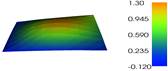
N=16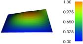
N=32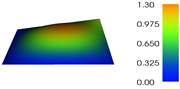
N=64
N=128

We plot in figure 1(a), the variation of log (e) and log (h) with increasing the number of cells N. We can see that both are decreasing with increasing the number of cells.

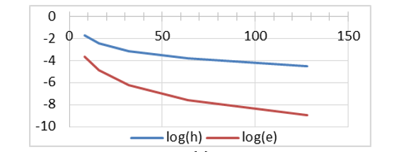
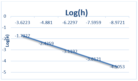
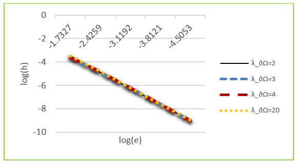
Figure 1 (b) represents the grid convergence, which estimates the order of the method numerically (the order is the slop of the curve), as we can see that the added Nitsche’s terms don’t degrade numerically the order of the method.

In Figure 1 (c), we represent the variation of log(e) with log(h) for different values of the stabilization parameter . As we can see the curves have the same shape and more or less the same values.

2.2. The Stokes Equation

Let  be a bounded domain in  with a smooth boundary .The stationary Stokes equation for a viscous incompressible flow, in dimensionless variables, can be written as:

With  is the velocity,  is the dynamic viscosity,  the pressure and  the external forces acting on the fluid.

The 2D exact solution of the Stokes problem can be taken

We are going to solve the Stokes problem, associated to Dirichlet Boundary conditions, numerically using the finite element method FEM, coupled with the Nitsche’s method for expressing the Dirichlet boundary conditions in Nitsche’s form. After that we compare the numerical results with the exact solution of the problem and calculate the error between them.

Let’s take first the weak formulation of the problem, with a viscosity equal to the unity. Dirichlet conditions are now enforced weakly using Nitsche's method by penalty-like terms and additional terms that maintain the skew-symmetry of the Stokes operator.

We use the Taylor Hood [11] setting and choose biquadratic finite element functions for the discrete velocity space and bilinear finite element functions for the discrete pressure space .Adding the skew symmetrisation, the penalty term  and the inflow stabilization . With  and  are the stabilization parameters.

For the simulation a rectangle domain with quadratic mesh is taken with length of 20 and width of 4  , , the number of cells  is going to be different in each case. Reynolds number will be constant during the simulation and will be equal to .

Symmetric formulation for the volumetric part

For this part we add terms forcing Dirichlet boundary conditions and then obtaining the Nitsche’s symmetric formulation of our problem.

With  trial functions and  test functions of our problem, with is the constant of parameterization and it’s taken equal to . denote the local mesh size and  the exact solution of the Stokes equation.

Skew-Symmetric formulation is:

We couple the classical formulation and the Nitsche’s formulation of the Stokes problem in the same running program.

We will use the well-known stabilizing technique [12] to handle the divergence constraint. The slip condition  is taken on the wall boundary of . This seems to be more practical than imposing it in strong form as that would involve both local coordinate transformations and the approximation of the normal at corners.

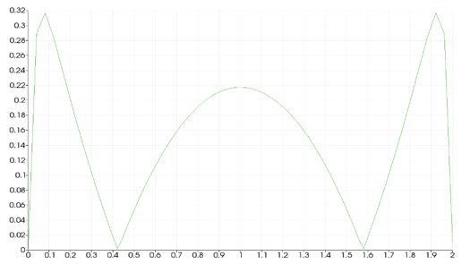
As we can see figure (2) represents the profile of velocity over vertical section in the middle of the domain and correspond to the shape of the given exact solution . We can see also that the free slip condition over the wall boundaries is respected and the value of the tangential velocity is not equal to zero.

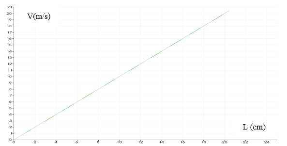
In figure (3) we can see the   increasing value of velocity when the flow is involving in the horizontal direction. And the graphic (4) represents the increasing value of the velocity in the central line of the domain.

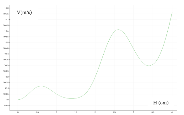
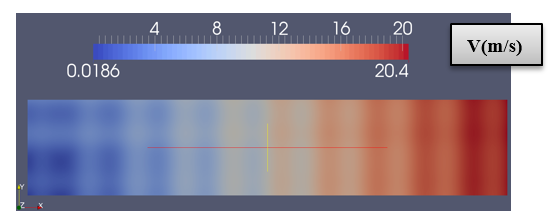
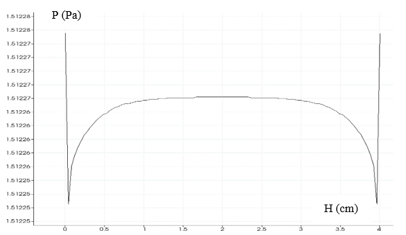
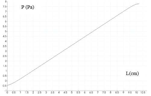
Figure 5 represents the graphic of pressure in a vertical section in the middle of the domain, the curve is in saddle shape.

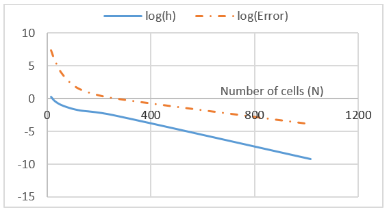
We obtain the following graphics Figure 6 (a) which represent the variation of the logarithmic value of the error and the logarithmic value of the mesh size in function of number of cells N. Then, we can see that the value of log(e) and log(h) are decreasing with increasing the number of cells N, which is first a confirmation of the fact that the Nitsche’s method is a mesh dependent method. Secondly, the error between the Nitsche’s method and the exact solution of the problem is really small and starts to be negligible if we increase the number of cells sufficiently.

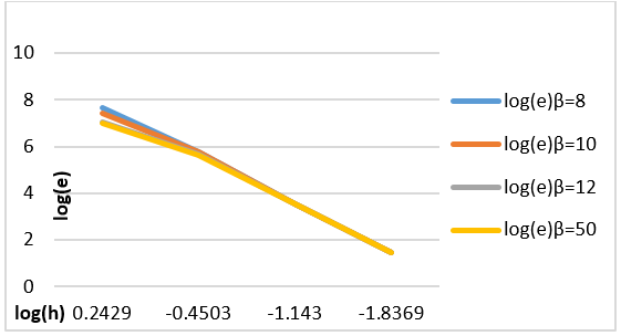
In Figure 6 (b) we give the representation of the variation of log(e) with log(h) for different values of the stabilization parameter .

2.3. Navier-Stokes Equation

We consider a two dimensional computational domain  with a boundary .The boundary is composed only on Dirichlet boundary condition.

The fluid velocity and the pressure of the flow problem is governed by the incompressible and isothermal Navier-Stokes equation. The Navier-Stokes equation and the mass conservation equation for an incompressible and isothermal flow are:

The internal stress tensor is defined as:

It is composed from the pressure  and a product of the dynamic viscosity denoted as and the strain rate tensor  given by

As Boundary conditions of the problem we take the inlet pressure constant and equal to . The inlet velocity is .

And  is the external volumetric forces acting on the fluid and its taken equal to 1, .The density is taken and the dynamic viscosity

Our domain  is a rectangle with quadratic mesh and it is taken with a length of 10 and a width of 2, and a number of cells equal to 2500.

In this section we are going to study the free slip boundary condition and the no slip boundary condition near to the wall boundary of the stationary Navier Stokes equation for an incompressible flow, using the Nitsche’s formulation for the Dirichlet boundary condition in each case.

2.3.1. Free Slip Case

Free slip case correspond to: and  at the wall boundary. It seems the normal component of the velocity is equal to zero and   the tangential component of the velocity is not equal to zero. We have kind of a drift flow at the wall boundary.

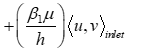
Nitsche’s formulation of the Dirichlet boundary conditions for the Navier Stokes equation in the free slip case is:

Volumetric part

To the volumetric terms we need to add Nitsche’s terms for all the Dirichlet boundaries of the domain with imposing the condition of free slip. Table III gives us different terms added to the bilinear and linear form for each boundary nature (Inlet, outlet and wall) of the domain to obtain   the final Nitsche’s formulation of the stationary Navier stokes equation.

After implementation of all these equations and running our program, we obtain the following results for the velocity and pressure.

3. Nitsche’s terms added to the linear and bilinear parts of the Navier-Stokes equation in free slip case.

Inlet
Terms added to a(u,v)
Terms added to L(v)
Outlet
Terms added to a(u,v)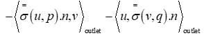
Terms added to L(v)
Wall
Terms added to a(u,v)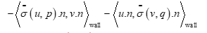
Terms added to L(v)

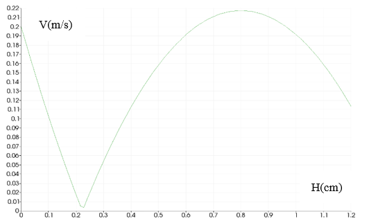
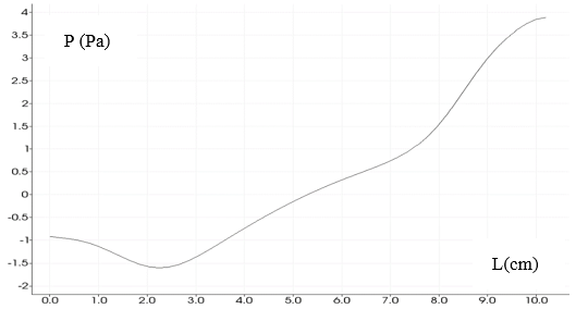
Figure 7(a) represents the graphic of velocity, as we can see the velocity is not equal to zero near to the wall boundaries as imposed. Figure 7(b) shows the variation of pressure in the central line along the geometry and the Figure 8 (a) represent the   distribution of velocity along the geometry, and the values are matching to the previous graphic.

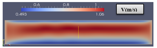
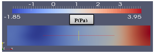
Figure 8 (b) represent the value of the pressure in the complete geometry. Negative values of the pressure represent the recirculation zones were we have tourbillons

2.3.2. No Slip Case

The no slip case corresponds to: and  at the wall boundary. We impose the zero velocity for both normal and tangential components. The Nitsche’s formulation of the Dirichlet boundary conditions will be different from the previous case.

Nitsche’s formulation for the no slip case:

The following table (Table IV) gives us different terms added to the bilinear and linear form for each boundary nature (Inlet, Outlet and Wall) of the domain to obtain the final Nitsche’s formulation of the stationary Navier-Stokes equation in the no slip case.

Table 4. Nitsche’s terms added to the linear and bilinear parts of the Navier-Stokes equation in the No-slip case.

Inlet
Terms added to a(u,v)
Terms added to L(v)
Outlet
Terms added to a(u,v)	No terms
Terms added to L(v)
Wall
Terms added to a(u,v)	No terms
Terms added to L(v)

As we can see, Figure 9 (a) represent the distribution of velocity in the domain, the value of the velocity at the wall is equal to zero, we can also see the important value of the velocity in opposite imposed flow direction near to the wall due to the recirculation of the flow in the opposite direction, we can see more details about the velocity direction in the Figure 9(b). Figure 10(a) represents a plot of velocity magnitude in a vertical section.

Figure 10(b) is a graphical representation of pressure values in a center line of the geometry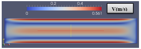

3. Conclusion

In this work, we gave a presentation of the Nitsche’s method and its application in different cases starting by the simple Poisson equation then the Stokes flow and finally the Navier-Stokes equation in both cases: slip and no slip boundary conditions. But, this is by no means the only field of application for the approach.

The Dirichlet boundary conditions were enforced weakly by using the Nitsche’s method. The error was calculated and we demonstrate through several numerical examples the performance and the robustness of the proposed variational form. The Nitsche’s method has a very wide range of application and it’s a very physical method. It employs only continuity conditions regarding the primal variable and the fluxes and simplify the variable coupling.

The only problem of the Nitsche’s method is to find the weak form. The generalization of the implementation for other problems is not as straightforward as for Lagrange multiplier method.

The choice of the stabilization parameters depends not only on the partial differential equation but also on the essential boundary condition. The choice of the stabilization parameters needs to be carefully made. This condition ensures the coercivity of the bilinear form in the interpolation space. Even in the case where there are not chosen rightly, the convergence is assured with a certain degree of convergence not far from the exact solution.

Regarding the choice of parameters, Nitsche’s method proved that if these parameters are taken with specific choice, then the discrete solution converges to the exact solution with optimal order. The advantage of this method is evident when we take into account the local mesh sizes.

An extension of the work will be done for the three dimensional problems, and implementation challenges are associated with the computational geometry and algorithmic aspects of implementation.

Acknowledgement

This work was supported by FRQNT (Fonds de Recherche Québécois en Nature et Technologie). The support is gratefully acknowledge.

References

[1] J. Nitsche, “Über ein Variationsprinzip zur Lösung von Dirichlet-Problemen bei Verwendung von Teilräumen, die keinen Randbedingungen unterworfen sind,” Abhandlungen aus dem mathematischen Seminar der Universität Hamburg, Springer, 1971. (In German) View Article
[2] I. Babuška, "The finite element method with Lagrangian multipliers," Numerische Mathematik, vol. 20, no. 3, pp. 179-192, 1973. View Article
[3] C. Kadapa, W. G. Ettmer, D. A. Peric, “Fictitious domain/distributed Lagrange multiplier based fluid–structure interaction scheme with hierarchical B-Spline grids,” Computer Methods in Applied Mechanics and Engineering, vol. 301, pp. 1-27, 2016. View Article
[4] P. Hansbo, A. Rashid, K. Salomonsson, “Least-squares stabilized augmented Lagrangian multiplier method for elastic contact,” Finite Elements in Analysis and Design, vol. 116, pp. 32-37, 2016. View Article
[5] R. Becker, R. Rannacher, “A feed-back approach to error control in finite element methods: basic analysis and examples,” East-West J. Numer. Math., vol. 4, pp. 237–264, 1996.
[6] P. Hansbo, C. Lovadina, I. Perugia, G. Sangalli, “A Lagrange multiplier method for the finite element solution of elliptic interface problems using non-matching meshes,” Numerische Mathematik, vol. 100, no. 1, pp. 91-115, 2005. View Article
[7] A. Johansson, M. Garzon, J. A. Sethian, “A three-dimensional coupled Nitsche and level set method for electrohydrodynamic potential flows in moving domains,” Journal of Computational Physics, vol. 309, pp. 88-111, 2016. View Article
[8] T. J. Truster, "A stabilized, symmetric Nitsche method for spatially localized plasticity,” Computational Mechanics, vol. 57, no. 1, pp. 75-103, 2016. View Article
[9] T. Rüberg, J. M. G. Aznar, “Numerical simulation of solid deformation driven by creeping flow using an immersed finite element method,” Advanced Modeling and Simulation in Engineering Sciences, 2016. View Article
[10] V. Thomée, Galerkin Finite Element Methods for Parabolic Problems. Springer, 1997. View Book
[11] J. Benk, M. Mehl, M. Ulbrich, “Sundance PDE solvers on Cartesian fixed grids in complex and variable geometries,” in Proceedings of ECCOMAS Thematic Conference on CFD and Optimization, Antalya, 2011. View Article
[12] L. P. Franca, T. J. R. Hughes, and R. Stenberg, Stabilized finite element methods for the Stokes problem, Incompressible Computational Fluid Dynamics-Trends and Advances (M. D. Gunzburger and R.A. Nicolaides, eds.). Cambridge University Press, 1993, pp. 87–107.