Journal of Fluid Flow, Heat and Mass Transfer (JFFHMT)

ISSN: 2368-6111

Nomenclature

• PWV: Pulse wave velocity (m/s)
• FSI: Fluid structure interaction
• : Volume (m³)
• : Variation, Del operator
• : Coefficients replacing the derivative of the function distributions
• : Flow behavior index
• : Axial normal and shear viscous stress (Pa)
• : Kinematic viscosity
• η: Nondimentional wall displacement
• : Density of incompressible fluid (kg/m³)
• : Function distribution in radial Direction for displacement and Velocity
• A: Cross sectional area (m²)
• C: Moens – Korteweg speed of Propagation (m/s)
• H, h: Thickness of the wall at a zero stress and loaded conditions respectively (m)
• : Action component for fluid and solid respectively
• K: Kinetic energy of the vessel wall (J)
• L, L_f: Lagrangian density functions for solids and solids, respectively.
• P: Pressure (Pa)
• R, r: Internal wall radii in zero stress & loaded conditions respectively (m)
• S: Entropy (J/K)
• t , T: Time (s), Temperature (K)
• u: Displacement vector (m)
• U, U_el,U_d: Internal, elastic and dissipative Energy (J)
• W_p: Work of external load (J)
• V: Velocity (m/s)

1. Introduction

Extensive work has been done for developing different models, applied to specific components of hemodynamic pulsating flow, such as arterial, venous and CSF circulations [1–4]. Functions of each component of the cardiovascular system and the relation of blood pressure to arterial disease predictions have been reviewed by Vosse and Stergiopulos – 2011 [1] and Quarteroni et al. – 2017 [5]. Numerical models are able to predict blood flow rate and pressure non-invasively and in a patient-specific setting, thus enabling non-invasive and less expensive disease diagnostics compared with clinical tests. Parker – 2009 [6], presents a historical review of arterial fluid mechanics models. Detailed derivation of simplified reduced Fluid – Structure Interaction (FSI) models for a linear elastic arterial system with account of visco-elasticity and inertia of the wall can be found in Peiro and Veneziani – 2009 [7]. Physical nonlinearity of thin and thick arterial walls coupled with large deformations have been introduced in FSI dynamics by Liberson et al. – 2016 [8] and Lillie et al. – 2016 [9]. An analytical solution for the pulse wave velocity (PWV) of a nonlinear FSI model was presented in Liberson et al. – 2014 [10]. The variational approach, yielding governing equations of physical phenomena, serves as an indispensable tool, when the interaction of the system components are non-trivial, for instance, when their interaction contain, strong nonlinearities, kinematic constraints, or high derivatives. The monumental book of Berdichevsky – 2010 [11,12] presents a variety of variational principles applied separately to fluids and solids. Kock and Olson – 1991 [13] developed a variational approach for FSI system, restricting analysis by a linear elastic thin-walled cylinder and an inviscid, irrotational and isentropic fluid flow. Lagrangian multipliers are used to enforce continuity equation constraint on boundary conditions. Multiple references can be found in this paper relating to the applications of the variational approach to the analysis of small vibrations of elastic bodies in a potential fluid. 

We demonstrate the effectiveness of Hamiltonian variational principle in analyzing FSI, without any limitations on dissipative fluid dynamics or physical properties of an adjacent flow path wall. We do not use the Lagrangian multiplier, accounting for the continuity equation explicitly, which simplifies the entire procedure. Internal boundary conditions are specified at junctions, including matching points in a combined 3D/1D approach, following from the Euler-Lagrange conditions.

Numerical effectiveness in a simulation of a pulsating flow is characterized by its ability to track a propagating wave for a few time periods, without suffering from numerical dissipation (errors in amplitude) or numerical dispersion (artificial oscillations). The most popular numerical methods in this area are the Lax-Wendroff finite volume method, its Taylor-Galerkin finite element counterpart, and discontinuous Galerkin spectral finite element method (As mentioned in [14]). Here, we also demonstrate the superior accuracy of the second order Total Variational Diminishing (TVD) approximation [15-17], compared to the more common Lax-Wendroff method. This higher accuracy can be essential when simulating a model with discontinuity in the load or material properties.

2. The Variational Principle for Fluid–Structure Interaction Problems

Hamilton’s variational principle is enunciated as a universal principle of nature unifying mechanical, thermodynamic, electromagnetic and other fields in a single least action functional, subject to extremization for a true process [11]. According to the mentioned principle, the variation of the action functional being applied to the FSI problem can be determined as:

Here  are variations of action components across fluid and solid volumes , ; t – time, -density of the fluid,  - the Lagrangian density functions for fluid and solids, respectively.

2.1. Fluid Domain

As mentioned by Berdichevsky - 2010 [11,12], variation of the Lagrangian density function in Eulerian coordinates can be written as follows:

Where – is a velocity vector,  – is internal energy as a function of density, S – entropy, – a distortion tensor (gradient of a displacement vector ), and T – temperature. Velocity, density and the displacement vector are not subject to independent variations. To avoid the use of Lagrangian multipliers, variation of density is directly extracted from the mass conservation law:

Presenting variation of a velocity as a substantial derivative of a variation of displacement vector, we have:

Equations (3) and (4) reduce the equation (2) to only the independent variables - displacement and entropy. Substituting (3) and (4) into equation (2) gives:

In which, according to Maxwell’s thermodynamic identity, pressure , and the stress tensor is introduced as .

Considering 2D axisymmetric flow in a long compliant tube, (i.e. long wave approximation [7]), we neglect variability of the radial velocity component and the pressure in radial direction. Thus, Equation (5) is transformed to the following form:

Here,  – is an axial velocity,  – is an axial component of displacement,  – axial normal and shear viscous stress components, - internal radius of a tube as a function of axial coordinate and time. The reduced models are based on assumptions regarding the  radial profiles, i.e.

With the aim of application to the incompressible flow, density is assumed constant. Integrating the functional (7) over the cross section with the following integration by parts, arrive at the reduced momentum equation

Where the coefficients are:

In case of Newtonian fluid (), generalized Hagen-Poiselle profile and a constant profile for the function distribution in radial direction,  equation (8) takes the form presented by San and Staples – 2012 [18].

Besides equation (8), Hamilton’s equation in a form of  yields natural boundary conditions. In case of a multiscale model, matching section of a coupled 3D and 1D require continuity following from natural boundary conditions

It should be noted that we neglect the effect of dissipation on boundary conditions.

2.2. Solid Domain

Consider a circular thin-wall cylinder relating to the polar system of coordinates.  Let  be the radius of the wall under the load,  – radius in a load free state,  - the wall thickness, – circumferential stretch ratio,  – nondimensionalized wall normal displacement. Introducing wall kinetic energy , elastic energy  and a dissipative energy  and work of external load , the Hamiltonian functional relating to the solid domain can be presented as

The normal velocity of the moving wall, defines kinetic energy per unit length

Internal elastic energy is composed of hyperelastic exponential strain energy (Fung, 1990 [19]) and an energy, accumulated by a longitudinal pre-stress force N, per unit area

Where , and  are material constants from Fung et al. anisotropic model [19]. Assuming the wall model is a system of independent nonlinearly elastic rings (Perktold and Rapitsch [20]), and simplifying the equation (14) by only keeping the principle quadratic terms (the forth power for  and quadratic terms for the slope), arrive at

Elementary work produced by the viscous component of circumferential stress, relating to the Voight type material and external pressure load are presented as

Substituting (13)-(16) into equation (12), and equating to zero, we obtain the equation of motion of an axisymmetric cylinder in the explicit form with respect to pressure

Momentum equation (8), equation of a boundary wall motion (17) and the continuity equation (3), averaged over the cross-section

Create a closed-form reduced mathematical model for fluid-structure interaction in a compliant channel.

3. Numerical Simulation

Numerical solvers utilized in a computational hemodynamics are typically based on the Lax-Wendroff scheme, its Taylor-Galerkin finite element counterpart, or a discontinuous Galerkin spectral finite element method [14]. In this article, the second-order accuracy monotonicity preserving TVD scheme is presented, which demonstrates its superiority for the problems dealing with a discontinuity of a load function, including discontinuity of its derivative, or material properties. This scheme can be applied to the linear scalar wave equation ( – is the unknown scalar function, a – coefficient)

The following numerical scheme (interested reader is referred to the book by Leveque [15]) has been applied

Here, the upper and lower indices correspond to the discrete time and a space coordinate, ,  is the limiter to maintain monotonicity ( for ).

The details of TVD methods applied to the arbitrary system of hyperbolic equations can be found in [15].  The following testing cases compare TVD and LW schemes.

3.1. Break-down Solution

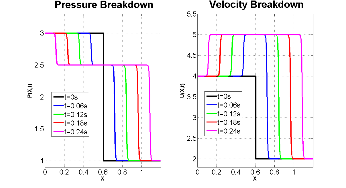
Numerical solution of the break-down problem (Riemann problem [14]) for the acoustics model, Equation (22), is simulated with the TVD (Figure 1) and the Lax-Wendroff (Figure 2) methods.

The solution was initialized with the piece-wise constant initial pressure and velocity data (shown by the black line in Figures 1 & 2). P and V values at the boundary were set to their constant initial values. The model runtime was set to stop before the wave front reach the boundaries. The same values of , , Courant number  and cell count of N was used for both schemes.  Discontinuity resolved by the TVD method, practically reproduces the exact solution (Figure 1), whereas discontinuity simulated by the Lax-Wendroff method gives rise to artificial oscillations (Figure 2). The Lax-Wendroff method is clearly dispersive, and does not perform well around discontinuities.

3.2. Single Segment Nonlinear FSI Problem

The nonlinear mathematical model used for this problem is based on the momentum equation (10) (α=1), continuity equation (18) and a linear constituent equation in the form of (17), accounting for the linear viscoelastic behavior of the wall. To generate this testing case, the method of manufactured solutions (MMS) [21,22] is used. We start by manufacturing an explicit expression for the solution as a superposition of Fourier harmonics, satisfying the corresponding linear equations. Then, we substitute the solution to the equations (10), (17) and (18), evaluating the source terms. Given the source terms, inlet velocity, exit pressure and initial conditions found from the exact solution, we use the simulation tool to obtain a numerical solution and compare it to the originally assumed solution with which we started. Results, presented in Figure 3 show that numerical and exact solutions of the nonlinear FSI problem, cannot be distinguished from one another in the pressure and veloc­­ity plots as a function of time. For smooth solutions (without the discontinuities), the Lax-Wendroff approach and TVD solutions give practically the same answer.

3.3. Bifurcated Elements Nonlinear FSI Problem

Schematic of a symmetric bifurcated structure with a single parent vessel and two identical daughter vessels (twins) are presented in Figure 4. We have manufactured an explicit expression for the solution as a superposition of three Fourier harmonics, satisfying a priori flow and pressure continuity at the matching sections.

The flow for the daughter and parent vessels are created such that the continuity condition at matching sections is satisfied automatically. , and  – is the local coordinate at each vessel, varying from 0 to  in daughter segment, and from 0 to in a parent vessel.

The following equations are used to specify flow at each interface (i.e. for parent or daughter vessels)

The pressure distributions for the parent, P_p (x,t),  and the daughter, P_d (x,t), vessels are manufactured providing automatic match  P_p (x=L_3,t)=P_d (x=0,t) at junctions (e.g. the gray colored area in Figure 4).

As mentioned before, we substitute the solution to the equations (10), (17) and (18), evaluating the source terms. Given the source terms, boundary and initial conditions just obtained, we use the simulation tool to obtain a numerical solution and compare it to the originally assumed solution with which we started. As presented in Figure 5, resulted P and V plots,  cannot be distinguished from one another in case of numerical (straight line) or  exact solution (square-dotted line). For smooth solutions, the Lax-Wendroff approach and TVD solutions give practically the same answer.

3.4. Sin-Wave Introduced in the Middle of the Parent Vessel in a Bifurcation

Lastly, the effectiveness of TVD scheme in preserving the shape of a propagating wave is evaluated by introducing a single Sin shape wave in the middle of the parent vessel. Figure 6 shows the propagation of this wave in a TVD based scheme compared to the Lax-Wendroff method. The flow properties similar to section 3.1, ρ=0.25 kg/m^3  , c=2 m/s, CFL=0.25 are used for both cases.

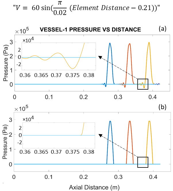
It can be seen that small oscillations exist in the left side of the sin wave in case of the Lax-Wendroff approximation. These oscillations (dispersion) increases as the sin wave propagates forward.

4. Conclusions

A general approach to derive the fluid-structure interaction problem have been applied based on Hamilton’s variational principle. Fluid is assumed viscous, and a boundary wall – nonlinear viscoelastic.  Internal boundary conditions at the matching sections of a multiscale 3D-1D approach are derived. Numerical results based on a TVD approach compared to the solutions provided by the Lax-Wendroff.  It is proved that the Lax-Wendroff method is clearly dispersive, providing artificially oscillations simulating physical problems with discontinuity. These oscillations are not present in TVD method, making it the optimum choice in solving 1D FSI problem. Derived internal boundary conditions enable the coupling of 1D FSI model to a local 3D FSI model of the arteries.

References

[1] F. N. van de Vosse, N. Stergiopulos, “Pulse Wave Propagation in the Arterial Tree,” Annu. Rev. Fluid Mech., vol. 43, no. 1, pp. 467–499, 2011. View Article
[2] B. A. Martin, P. Reymond, J. Novy, O. Balédent, N. Stergiopulos, “A Coupled Hydrodynamic Model of the Cardiovascular and Cerebrospinal Fluid System,” Am. J. Physiol. Heart Circ. Physiol., vol. 302, no. 7, pp. H1492-H1509, 2012. View Article
[3] L. O. Muller, “Mathematical Modelling and Simulation of the Human Circulation with Emphasis on the Venous System: Application to the CCSVI Condition,” Ph.D. dissertation, University of Trento, Trento, Italy, 2014. View Publication
[4] S. Gupta, M. Soellinger, D. M. Grzybowski, P. Boesiger, J. Biddiscombe, D. Poulikakos, V. Kurtcuoglu, “Cerebrospinal Fluid Dynamics in the Human Cranial Subarachnoid Space: An Overlooked Mediator of Cerebral Disease. I. Computational Model,” J. R. Soc. Interface, vol. 7, no. 49, pp. 1195–1204, 2010. View Article
[5] A. Quarteroni, A. Manzoni, C. Vergara, “The Cardiovascular System: Mathematical Modelling, Numerical Algorithms and Clinical Applications,” Acta Numer., vol. 26, pp. 365–590, 2017. View Article
[6] K. H. Parker, “A Brief History of Arterial Wave Mechanics,” Med. Biol. Eng. Comput., vol. 47, no. 2, pp. 111–118, 2009. View Article
[7] J. Peiró, A. Veneziani, “Reduced Models of the Cardiovascular System,” in Cardiovascular Mathematics, L. Formaggia, A. Quarteroni, and A. Veneziani, Eds., Milan: Springer, pp. 347–394. View Article
[8] A. S. Liberson, J. S. Lillie, S. W. Day, D. A. Borkholder, “A Physics Based Approach to the Pulse Wave Velocity Prediction in Compliant Arterial Segments,” J. Biomech., vol. 49, no. 14, pp. 3460–3466, 2016. View Article
[9] J. S. Lillie, A. S. Liberson, D. A. Borkholder, “Quantification of Hemodynamic Pulse Wave Velocity Based on a Thick Wall Multi-Layer Model for Blood Vessels,” J. Fluid Flow Heat Mass Transf. JFFHMT, vol. 3, no. 1, pp. 54–61, 2016. View Article
[10] A. S. Liberson, J. S. Lillie, D. A. Borkholder, “Numerical Solution for the Boussinesq Type Models with Application to Arterial Flow,” J. Fluid Flow Heat Mass Transf., vol. 1, pp. 9-15, 2014. View Article
[11] V. L. Berdichevsky, “Variational Principles,” in Variational Principles of Continuum Mechanics, Berlin, Heidelberg: Springer, pp. 3–44, 2009. View Book
[12] V. L. Berdichevsky, “Steady Motion of Ideal Fluid and Elastic Body,” in Variational Principles of Continuum Mechanics, Berlin, Heidelberg: Springer, pp. 473–494, 2009. View Book
[13] E. Kock, L. Olson, “Fluid-Structure Interaction Analysis by the Finite Element Method–a Variational Approach,” Int. J. Numer. Methods Eng., vol. 31, no. 3, pp. 463–491, 1991. View Article
[14] L. Formaggia, A. Quarteroni, A. Veneziani, Cardiovascular Mathematics - Modeling and Simulation of the Circulatory System. Milano: Springer, 2009. View Book
[15] R. Leveque, Finite Volume Methods for Hyperbolic Problems. Cambridge: University Press, 2002. View Book
[16] Y. Kosolapov, A. Liberson “An implicit relaxation method for computation of 3D flows of spontaneously condensing steam” Computational mathematics and mathematical physics., vol. 37, no. 6, pp. 759-768, 1997.
[17] A. Liberson, S. Hesler, T. Mc.Closkey, “Inviscid and viscous numerical simulation for non-equilibrium spontaneously condensing flows in steam turbine blade passages,” PWR-Vol.33, 1998 International Joint Power Generation Conference. vol. 2, ASME 1998, pp.97-105.
[18] O. San, A. Staples, “An improved model for reduced order physiological fluid flows,” Journal of Mechanics in Medicine and Biology, vol. 12, no. 3, pp.1-37, 2012. View Article
[19] Y. C. Fung, K. Fronek, P. Patitucci, “Pseudoelasticity of arteries and the choice of its mathematical expression,” Am. J. Physiol., vol. 237, no. 5, pp. H620–31, 1979. View Article
[20] K. Perktold, G, Rappitsch, “Computer Simulation of Local Blood Flow and Vessel Mechanics in a Compliant Carotid Artery Bifurcation Model,” J. Biomech., vol. 28, no. 7, pp. 845–856, 1995. View Article
[21] C. J. Roy, “Review of Code and Solution Verification Procedures for Computational Simulation,” J. Comput. Phys., vol. 205, no. 1, pp. 131–156, 2005. View Article
[22] L. Shunn, F. Ham, “Method of Manufactured Solutions Applied to Variable-Density Flow Solvers,” In: Annual Research Briefs, Center for Turbulence Research, pp. 155–168, 2007. View Article